R: 4.3.2 (2023-10-31)
R studio: 2023.12.1+402 (2023.12.1+402)
Marketing Effectiveness and Resource Allocation
Leverage historical data to quantify the effectiveness of marketing actions.
1
2
3
4
5
6
7
8
9
| > spending.data <- read_xls("advertising spending 1.xls")
> str(spending.data)
tibble [200 × 5] (S3: tbl_df/tbl/data.frame)
$ week : num [1:200] 1 2 3 4 5 6 7 8 9 10 ...
$ tv : num [1:200] 230.1 44.5 17.2 151.5 180.8 ...
$ radio : num [1:200] 37.8 39.3 45.9 41.3 10.8 48.9 32.8 19.6 2.1 2.6 ...
$ newspaper: num [1:200] 69.2 45.1 69.3 58.5 58.4 75 23.5 11.6 1 21.2 ...
$ sales : num [1:200] 22.1 10.4 9.3 18.5 12.9 7.2 11.8 13.2 4.8 10.6 ...
|
数据包含每周的销售额以及电视、广播和报纸广告费用(以千英镑计)。
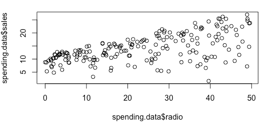
Does radio advertising affect sales for an electronics brand?
Visualizing the data
1
2
| ## scatter plot
plot(spending.data$radio, spending.data$sales)
|
 1
 2
 3
 4
 5
 6
 7
 8
 9
10
11
12
13
14
15
16
17
18
19
20
21
22
23
24
25
| > # Correlation between radio advertising and sales
> cor(spending.data$radio, spending.data$sales)
[1] 0.5762226
> regression <- lm(sales ~ radio, data = spending.data)
> summary(regression)
Call:
lm(formula = sales ~ radio, data = spending.data)
Residuals:
Min 1Q Median 3Q Max
-15.7305 -2.1324 0.7707 2.7775 8.1810
Coefficients:
Estimate Std. Error t value Pr(>|t|)
(Intercept) 9.31164 0.56290 16.542 <2e-16 ***
radio 0.20250 0.02041 9.921 <2e-16 ***
---
Signif. codes: 0 ‘***’ 0.001 ‘**’ 0.01 ‘*’ 0.05 ‘.’ 0.1 ‘ ’ 1
Residual standard error: 4.275 on 198 degrees of freedom
Multiple R-squared: 0.332, Adjusted R-squared: 0.3287
F-statistic: 98.42 on 1 and 198 DF, p-value: < 2.2e-16
|
问题:如果我在广播广告上花费 40,000 英镑,我将卖出多少?答案:17.31 = 9.31 +0.20 * 40
Accounting for multiple predictors: multiple linear regression
 1
 2
 3
 4
 5
 6
 7
 8
 9
10
11
12
13
14
15
16
17
18
19
20
21
22
| > regression <- lm(sales ~ radio + tv, data=spending.data)
> summary(regression)
Call:
lm(formula = sales ~ radio + tv, data = spending.data)
Residuals:
Min 1Q Median 3Q Max
-8.7977 -0.8752 0.2422 1.1708 2.8328
Coefficients:
Estimate Std. Error t value Pr(>|t|)
(Intercept) 2.92110 0.29449 9.919 <2e-16 ***
radio 0.18799 0.00804 23.382 <2e-16 ***
tv 0.04575 0.00139 32.909 <2e-16 ***
---
Signif. codes: 0 ‘***’ 0.001 ‘**’ 0.01 ‘*’ 0.05 ‘.’ 0.1 ‘ ’ 1
Residual standard error: 1.681 on 197 degrees of freedom
Multiple R-squared: 0.8972, Adjusted R-squared: 0.8962
F-statistic: 859.6 on 2 and 197 DF, p-value: < 2.2e-16
|
Allocating marketing budgets
Ratio of elasticities method
- What is elasticity?
- % change in the response variable for a 1% change in the predictor variable
- Example: the % change in sales for a 1% change in advertising spending
Let us start with an example:
- Image that you have a £100,000 budget to spend on advertising
- A 1% increase in online advertising increases sales by 0.12%
- A 1% increase in offline advertising increases sales by 0.08%
如何使用弹性系数法?
- 总弹性系数:0.12 + 0.08 = 0.20。
- 弹性系数比率:
- 在线广告:0.12/0.20 = 60%
- 线下广告:0.08/0.20 = 40%
建议:将60%(£60,000)的预算分配给在线广告,40%(£40,000)的预算分配给线下广告。
How to obtain elasticities from a linear regression model?
- 广告弹性 = 广告估算值 * (基线广告/基线销售)
- 基线广告 = 平均广播广告支出(=23.26)
- Baseline Sales = average sales (=14.02)
- What is the elasticity of radio advertising? (0.32)
- A 1% increase in radio advertising results in a 0.32% increase in sales.
1
2
3
4
5
6
7
8
| > mean(spending.data$radio)
[1] 23.264
> mean(spending.data$sales)
[1] 14.0225
> 0.19 * (23.26/14.02)
[1] 0.3152211
|
Marketing Mix Modelling
Modelling non-linear returns on investment
假设广告在初始预算为50万英镑的情况下在1周内播出,旨在提高英国消费者对Airbnb作为一个包容性品牌的认知,同时增加访问Airbnb网站和预订的流量。
由于该广告活动的结果,Airbnb的预订量增加了1%。
一年后,Airbnb决定再次进行一场相似的广告活动,同样持续1周,但将预算翻倍至100万英镑,希望预订量会增加2%。
你认为会发生这种情况吗?为什么(为什么不)?
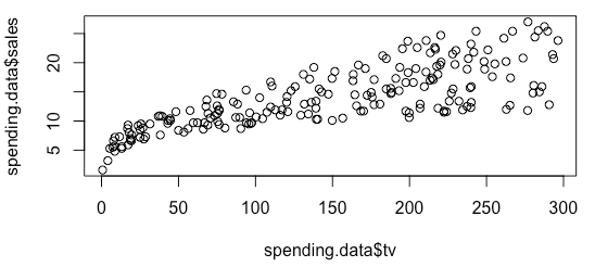
“电视和广告之间的关系是否线性?”
1
| plot(spending.data$tv, spending.data$sales)
|
 1
 2
 3
 4
 5
 6
 7
 8
 9
10
11
12
13
14
15
16
17
18
19
20
21
22
23
24
25
26
27
28
29
30
31
32
33
34
35
36
37
38
39
40
| > summary(spending.data$sales)
Min. 1st Qu. Median Mean 3rd Qu. Max.
1.60 10.38 12.90 14.02 17.40 27.00
> summary(spending.data$tv)
Min. 1st Qu. Median Mean 3rd Qu. Max.
0.70 74.38 149.75 147.04 218.82 296.40
> summary(spending.data$radio)
Min. 1st Qu. Median Mean 3rd Qu. Max.
0.000 9.975 22.900 23.264 36.525 49.600
> summary(spending.data$newspaper)
Min. 1st Qu. Median Mean 3rd Qu. Max.
0.30 12.75 25.75 30.55 45.10 114.00
> regression <- lm(log(sales) ~ log(radio+0.01) + log(tv) + log(newspaper), data=spending.data)
> summary(regression)
Call:
lm(formula = log(sales) ~ log(radio + 0.01) + log(tv) + log(newspaper),
data = spending.data)
Residuals:
Min 1Q Median 3Q Max
-0.45346 -0.08881 -0.01746 0.06781 0.78863
Coefficients:
Estimate Std. Error t value Pr(>|t|)
(Intercept) 0.479773 0.052031 9.221 <2e-16 ***
log(radio + 0.01) 0.144177 0.007865 18.333 <2e-16 ***
log(tv) 0.349297 0.008857 39.437 <2e-16 ***
log(newspaper) 0.017488 0.009306 1.879 0.0617 .
---
Signif. codes: 0 ‘***’ 0.001 ‘**’ 0.01 ‘*’ 0.05 ‘.’ 0.1 ‘ ’ 1
Residual standard error: 0.1254 on 196 degrees of freedom
Multiple R-squared: 0.9098, Adjusted R-squared: 0.9084
F-statistic: 658.7 on 3 and 196 DF, p-value: < 2.2e-16
|
我们已经将0.01添加到广播的值上,因为广播的最小值是0,这样做会导致对log(广播)的无效结果。
1
2
3
4
5
6
7
8
9
| Linear
• Equation: Y = β0 + β1X
• Interpretation: One unit change in X leads to beta1 unit change in Y
• When to use? Linear relation between X and Y
Log-Log
• Equation: log(Y) = β0 + β1log(X)
• Interpretation: One percent change in X leads to β1 percent change in Y • When to use? A non-linear relation between X and Y
Which one to use?
• Plot the data to learn about the relation between X and Y. • Estimate both models and identify the best fitting model
|
- 营销组合工具的综合使用可以产生协同效应。
- 当多种媒体的联合影响超过它们各自部分的总和时,就会产生协同效应。
Is TV advertising more effective in the presence of radio advertising?
 1
 2
 3
 4
 5
 6
 7
 8
 9
10
11
12
13
14
15
16
17
18
19
20
21
22
23
24
25
| > regression <- lm(log(sales) ~ log(radio+0.01) + log(tv) + log(newspaper) + log(radio+0.01)*log(tv), data=spending.data)
> summary(regression)
Call:
lm(formula = log(sales) ~ log(radio + 0.01) + log(tv) + log(newspaper) +
log(radio + 0.01) * log(tv), data = spending.data)
Residuals:
Min 1Q Median 3Q Max
-0.29117 -0.06889 -0.02084 0.05787 0.74453
Coefficients:
Estimate Std. Error t value Pr(>|t|)
(Intercept) 1.347498 0.101811 13.235 < 2e-16 ***
log(radio + 0.01) -0.152661 0.032200 -4.741 4.10e-06 ***
log(tv) 0.153799 0.022032 6.981 4.49e-11 ***
log(newspaper) 0.019947 0.007741 2.577 0.0107 *
log(radio + 0.01):log(tv) 0.066311 0.007043 9.415 < 2e-16 ***
---
Signif. codes: 0 ‘***’ 0.001 ‘**’ 0.01 ‘*’ 0.05 ‘.’ 0.1 ‘ ’ 1
Residual standard error: 0.1043 on 195 degrees of freedom
Multiple R-squared: 0.938, Adjusted R-squared: 0.9367
F-statistic: 737 on 4 and 195 DF, p-value: < 2.2e-16
|
使用中心化变量
 1
 2
 3
 4
 5
 6
 7
 8
 9
10
11
12
13
14
15
16
17
18
19
20
21
22
23
24
25
26
27
28
29
30
31
32
| > center <- function(x) { scale(x, scale = F)} # scale = F, means only center not standardize
> spending.data <- spending.data %>% mutate(radio_log_centered = center(log(radio+0.01)),
+ tv_log_centered .... [TRUNCATED]
> regression <- lm(log(sales) ~ radio_log_centered + tv_log_centered + newspaper_log_centered +
+ radio_log_centered*tv_log_centere .... [TRUNCATED]
> summary(regression)
Call:
lm(formula = log(sales) ~ radio_log_centered + tv_log_centered +
newspaper_log_centered + radio_log_centered * tv_log_centered,
data = spending.data)
Residuals:
Min 1Q Median 3Q Max
-0.29117 -0.06889 -0.02084 0.05787 0.74453
Coefficients:
Estimate Std. Error t value Pr(>|t|)
(Intercept) 2.561748 0.007376 347.306 <2e-16 ***
radio_log_centered 0.157146 0.006681 23.521 <2e-16 ***
tv_log_centered 0.337076 0.007476 45.086 <2e-16 ***
newspaper_log_centered 0.019947 0.007741 2.577 0.0107 *
radio_log_centered:tv_log_centered 0.066311 0.007043 9.415 <2e-16 ***
---
Signif. codes: 0 ‘***’ 0.001 ‘**’ 0.01 ‘*’ 0.05 ‘.’ 0.1 ‘ ’ 1
Residual standard error: 0.1043 on 195 degrees of freedom
Multiple R-squared: 0.938, Adjusted R-squared: 0.9367
F-statistic: 737 on 4 and 195 DF, p-value: < 2.2e-16
|
Modelling carryover effects
到目前为止,我们假设在给定时间段内的广告只会影响该时间段内的销售。实际上,消费者对广告的反应可能会有延迟。不考虑延迟效应可能会导致广告弹性系数被低估。
广告存量度量了广告在当前时间段之外的影响。
广告存量背后的理论是,营销曝光在消费者心中建立了意识。这种意识不会在消费者看到广告后立即消失,而是留存在他们的记忆中。记忆会随着时间的推移而减弱,因此广告存量中存在衰减部分。
1
| Adstockt = Advertisingt + λAdstockt−1
|
在每个时间段中,你被认为会保留前一个广告存量的一部分(λ)。
例如,如果λ等于0.3,则来自一个时间段之前的广告存量在当前时间段仍然具有30%的影响。
How to do this in R?
- “rate = 0.1” sets λ to 0.1 (i.e. 10%)
- You can empirically test multiple values of λ.
 1
 2
 3
 4
 5
 6
 7
 8
 9
10
11
12
13
14
15
16
17
18
19
20
21
22
23
24
25
26
27
28
29
30
31
32
| > adstock <- function(x, rate){
+ return(as.numeric(stats::filter(x=x, filter=rate, method="recursive")))
+ }
> # filter() function from stats package applies linear filtering to a univariate time series
>
> spending.data <- spending.data %>% mutate(tv_adstoc .... [TRUNCATED]
> regression <- lm(log(sales) ~ log(radio+0.01) + log(tv_adstock) + log(newspaper), data=spending.data)
> summary(regression)
Call:
lm(formula = log(sales) ~ log(radio + 0.01) + log(tv_adstock) +
log(newspaper), data = spending.data)
Residuals:
Min 1Q Median 3Q Max
-0.96605 -0.08394 -0.00081 0.07966 0.81860
Coefficients:
Estimate Std. Error t value Pr(>|t|)
(Intercept) -0.09547 0.08418 -1.134 0.2581
log(radio + 0.01) 0.13177 0.01008 13.074 <2e-16 ***
log(tv_adstock) 0.45582 0.01542 29.567 <2e-16 ***
log(newspaper) 0.02219 0.01190 1.865 0.0637 .
---
Signif. codes: 0 ‘***’ 0.001 ‘**’ 0.01 ‘*’ 0.05 ‘.’ 0.1 ‘ ’ 1
Residual standard error: 0.1604 on 196 degrees of freedom
Multiple R-squared: 0.8523, Adjusted R-squared: 0.8501
F-statistic: 377.1 on 3 and 196 DF, p-value: < 2.2e-16
|
Predictive accuracy *
 1
 2
 3
 4
 5
 6
 7
 8
 9
10
11
12
13
14
15
16
17
18
19
20
21
22
23
24
25
26
27
28
29
30
31
32
33
34
35
| > # Total number of rows in the data frame
> n <- nrow(spending.data)
> # Number of rows for the training set (80% of the dataset)
> n_train <- round(0.80 * n) # Training data
> spending.data.train <- subset(spending.data, week <= n_train) # Holdout data
> spending.data.holdout <- subset(spending.data, week > n_train)
> # Estimation on training data
> regression <- lm(log(sales) ~ log(radio_adstock) + log(tv_adstock) + log(newspaper_adstock), data=spending.data.trai .... [TRUNCATED]
> summary(regression)
Call:
lm(formula = log(sales) ~ log(radio_adstock) + log(tv_adstock) +
log(newspaper_adstock), data = spending.data.train)
Residuals:
Min 1Q Median 3Q Max
-0.95544 -0.06206 -0.00140 0.07359 0.60782
Coefficients:
Estimate Std. Error t value Pr(>|t|)
(Intercept) -0.37264 0.09377 -3.974 0.000108 ***
log(radio_adstock) 0.19215 0.01473 13.048 < 2e-16 ***
log(tv_adstock) 0.47022 0.01566 30.031 < 2e-16 ***
log(newspaper_adstock) 0.02057 0.01545 1.332 0.184852
---
Signif. codes: 0 ‘***’ 0.001 ‘**’ 0.01 ‘*’ 0.05 ‘.’ 0.1 ‘ ’ 1
Residual standard error: 0.1483 on 156 degrees of freedom
Multiple R-squared: 0.8812, Adjusted R-squared: 0.8789
F-statistic: 385.6 on 3 and 156 DF, p-value: < 2.2e-16
|
 1
 2
 3
 4
 5
 6
 7
 8
 9
10
11
12
| > # Predict sales on holdout data
> spending.data.holdout$predicted_sales_log <-
+ predict(object =regression, newdata = spending.data.holdout)
> # Convert predicted log sales to actual sales
> spending.data.holdout$predicted_sales <- exp(spending.data.holdout$predicted_sales_log)
> # Quantify predictive accuracy: Mean Average Percentage Error (MAPE)
> mape <- mean(abs((spending.data.holdout$sales -spending.data.holdout$predicte .... [TRUNCATED]
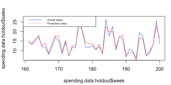
> mape # Reflects the average percentage error in a given week
[1] 0.1010304
|
1
2
3
4
5
6
| > # Plot actual versus predicted sales
> plot(spending.data.holdout$week, spending.data.holdout$sales, type="l", col="blue") # Plot actual sales
> lines(spending.data.holdout$week,spending.data.holdout$predicted_sales, type = "l", col = "red") # Add predicted sales
> legend("topleft", legend=c("Actual sales", "Predicted sales"), col=c("blue", "red"), lty = 1:2, cex=0.6)
|