R: 4.3.2 (2023-10-31)
R studio: 2023.12.1+402 (2023.12.1+402)

1. Manage customer hierarchical

1.1 segmentation

According to the demographics data provided, ‘Emplyment’ data was excluded because it was related to salary. The data with ‘salary=7’ was removed because it was invalid. ‘Regions’ are simplified to 3. Finally the continuous vectors are normalized and the ordinal variables are factored.

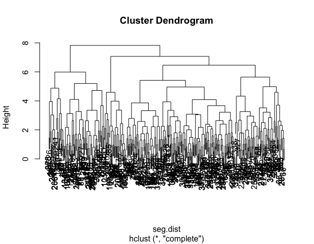
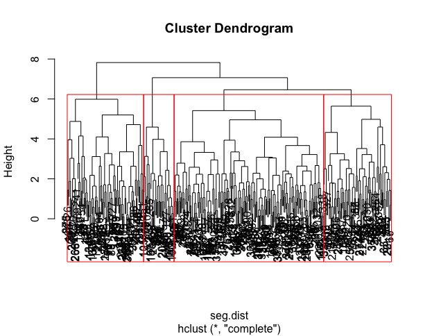
Considering data contains ordinal varibles and continous variables, we segment customers into four groups based on hierarchical clustering, which differentiation between groups was more appropriate than three or five groups.

1.1.1 import and check data

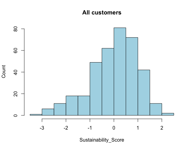
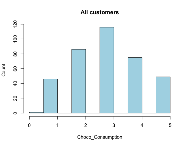
> seg.df <- read.csv("1_demographics.csv", stringsAsFactors = TRUE)
> head(seg.df, n = 5)
Consumer_id Age_Group Gender Salary Education Employment Location_by_region Choco_Consumption
1 352 1 2 1 2 3 4 0
2 103 3 2 3 1 1 1 1
3 17 1 1 1 1 4 1 1
4 66 1 1 1 1 3 1 1
5 329 2 1 1 1 8 1 1
Sustainability_Score
1 -1.15059
2 0.50287
3 -1.14517
4 -0.46688
5 -2.08817
> summary(seg.df, digits = 2)
Consumer_id Age_Group Gender Salary Education Employment Location_by_region
Min. : 1 Min. :1.0 Min. :1.0 Min. :0.0 Min. :1.0 Min. : 1.0 Min. :1.0
1st Qu.: 95 1st Qu.:1.0 1st Qu.:1.0 1st Qu.:1.0 1st Qu.:2.0 1st Qu.: 1.0 1st Qu.:1.0
Median :190 Median :2.0 Median :2.0 Median :2.0 Median :2.0 Median : 2.0 Median :1.0
Mean :190 Mean :2.2 Mean :1.7 Mean :2.3 Mean :2.3 Mean : 2.4 Mean :1.3
3rd Qu.:284 3rd Qu.:3.0 3rd Qu.:2.0 3rd Qu.:3.0 3rd Qu.:3.0 3rd Qu.: 3.0 3rd Qu.:1.0
Max. :378 Max. :4.0 Max. :2.0 Max. :7.0 Max. :4.0 Max. :10.0 Max. :8.0
Choco_Consumption Sustainability_Score
Min. :0 Min. :-3.26
1st Qu.:2 1st Qu.:-0.61
Median :3 Median : 0.14
Mean :3 Mean : 0.00
3rd Qu.:4 3rd Qu.: 0.68
Max. :5 Max. : 2.04
>
> ### 1.1.1 remove consumer_id in data set, and set consumer_id as row name
> rownames(seg.df) <- seg.df[, 1]
> seg.df <- seg.df[, -1]
> #### remove salary = 7, invalid data
> seg.df <- seg.df[seg.df$Salary != 7, ]
> #### remove Employment, which related to Salary
> seg.df <- subset(seg.df, select = -Employment)
> #### just split region to 3 groups
> seg.df$Location_by_region[seg.df$Location_by_region > 2] <- 3
hist(seg.df$Sustainability_Score,
main = "All customers",
xlab = "Sustainability_Score",
ylab = "Count",
col = "lightblue" # colore the bars
)
hist(seg.df$Choco_Consumption,
main = "All customers",
xlab = "Choco_Consumption",
ylab = "Count",
col = "lightblue" # colore the bars
)
> head(seg.df, n = 5)
Age_Group Gender Salary Education Location_by_region Choco_Consumption Sustainability_Score
352 1 2 1 2 3 0 -1.15059
103 3 2 3 1 1 1 0.50287
17 1 1 1 1 1 1 -1.14517
66 1 1 1 1 1 1 -0.46688
329 2 1 1 1 1 1 -2.08817
> summary(seg.df, digits = 2)
Age_Group Gender Salary Education Location_by_region Choco_Consumption
Min. :1.0 Min. :1.0 Min. :0.0 Min. :1.0 Min. :1.0 Min. :0
1st Qu.:1.0 1st Qu.:1.0 1st Qu.:1.0 1st Qu.:2.0 1st Qu.:1.0 1st Qu.:2
Median :2.0 Median :2.0 Median :2.0 Median :2.0 Median :1.0 Median :3
Mean :2.1 Mean :1.7 Mean :2.2 Mean :2.3 Mean :1.2 Mean :3
3rd Qu.:3.0 3rd Qu.:2.0 3rd Qu.:3.0 3rd Qu.:3.0 3rd Qu.:1.0 3rd Qu.:4
Max. :4.0 Max. :2.0 Max. :6.0 Max. :4.0 Max. :3.0 Max. :5
Sustainability_Score
Min. :-3.3e+00
1st Qu.:-6.1e-01
Median : 1.4e-01
Mean :-9.6e-05
3rd Qu.: 6.8e-01
Max. : 2.0e+00
> str(seg.df)
'data.frame': 373 obs. of 7 variables:
$ Age_Group : int 1 3 1 1 2 4 2 1 1 1 ...
$ Gender : int 2 2 1 1 1 1 2 2 1 1 ...
$ Salary : int 1 3 1 1 1 4 2 3 3 3 ...
$ Education : int 2 1 1 1 1 1 1 2 2 2 ...
$ Location_by_region : num 3 1 1 1 1 1 1 1 1 1 ...
$ Choco_Consumption : int 0 1 1 1 1 1 1 1 1 1 ...
$ Sustainability_Score: num -1.151 0.503 -1.145 -0.467 -2.088 ...

> seg.df.sc <- seg.df
> #### just scale continous variables
> seg.df.sc[, c(6,7)] <- scale(seg.df[ , c(6,7)])
> #### factor ordered ordinals
> seg.df.sc$Age_Group <- factor(seg.df.sc$Age_Group, ordered = TRUE)
> seg.df.sc$Salary <- factor(seg.df.sc$Salary, ordered = TRUE)
> seg.df.sc$Education <- factor(seg.df.sc$Education, ordered = TRUE)
> seg.df.sc$Gender <- factor(seg.df.sc$Gender, ordered = FALSE)
> seg.df.sc$Location_by_region <- factor(seg.df.sc$Location_by_region, ordered = FALSE)
> head(seg.df.sc, n = 5)
Age_Group Gender Salary Education Location_by_region Choco_Consumption Sustainability_Score
352 1 2 1 2 3 -2.449983 -1.1457402
103 3 2 3 1 1 -1.627442 0.5008876
17 1 1 1 1 1 -1.627442 -1.1403426
66 1 1 1 1 1 -1.627442 -0.4648553
329 2 1 1 1 1 -1.627442 -2.0794461
> summary(seg.df.sc, digits = 2)
Age_Group Gender Salary Education Location_by_region Choco_Consumption Sustainability_Score
1:140 1:119 0: 34 1: 76 1:299 Min. :-2.450 Min. :-3.25
2:120 2:254 1:116 2:183 2: 58 1st Qu.:-0.805 1st Qu.:-0.61
3: 35 2: 40 3: 43 3: 16 Median : 0.018 Median : 0.14
4: 78 3:123 4: 71 Mean : 0.000 Mean : 0.00
4: 41 3rd Qu.: 0.840 3rd Qu.: 0.68
5: 14 Max. : 1.663 Max. : 2.03
6: 5
> str(seg.df.sc)
'data.frame': 373 obs. of 7 variables:
$ Age_Group : Ord.factor w/ 4 levels "1"<"2"<"3"<"4": 1 3 1 1 2 4 2 1 1 1 ...
$ Gender : Factor w/ 2 levels "1","2": 2 2 1 1 1 1 2 2 1 1 ...
$ Salary : Ord.factor w/ 7 levels "0"<"1"<"2"<"3"<..: 2 4 2 2 2 5 3 4 4 4 ...
$ Education : Ord.factor w/ 4 levels "1"<"2"<"3"<"4": 2 1 1 1 1 1 1 2 2 2 ...
$ Location_by_region : Factor w/ 3 levels "1","2","3": 3 1 1 1 1 1 1 1 1 1 ...
$ Choco_Consumption : num -2.45 -1.63 -1.63 -1.63 -1.63 ...
$ Sustainability_Score: num -1.146 0.501 -1.14 -0.465 -2.079 ...

1.1.2 hclust()

Considering data contains ordinal varibles and continous variables, use hclust().

> ### 1.1.2 Hierarchical clustering: hclust()
> seg.dist <- dist(seg.df.sc)
> # seg.dist <- daisy(seg.df.sc, metric = "gower")
> as.matrix(seg.dist)[1:7, 1:7]
352 103 17 66 329 241 34
352 0.000000 4.048204 2.5839125 2.6721113 2.923762 4.977689 2.821760
103 4.048204 0.000000 3.4195960 3.1516122 3.557825 2.618749 1.799080
17 2.583913 3.419596 0.0000000 0.6754873 1.371829 4.254911 1.811081
66 2.672111 3.151612 0.6754873 0.0000000 1.899185 4.358532 1.738220
329 2.923762 3.557825 1.3718292 1.8991849 0.000000 3.657826 2.038581
241 4.977689 2.618749 4.2549114 4.3585316 3.657826 0.000000 3.118659
34 2.821760 1.799080 1.8110812 1.7382205 2.038581 3.118659 0.000000
> seg.hc <- hclust(seg.dist, method="complete")
> plot(seg.hc)
> rect.hclust(seg.hc, k=4, border = "red")
> seg.hc.segment <- cutree(seg.hc, k=4) #membership vector for 4 groups 
> table(seg.hc.segment) #counts
seg.hc.segment
1 2 3 4
78 172 88 35

data size of groups

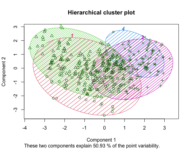
> clusplot(seg.df, seg.hc.segment,
+ color = TRUE, #color the groups
+ shade = TRUE, #shade the ellipses for group membership
+ labels = 4, #label only the groups, not the individual points
+ lines = 0, #omit distance lines between groups
+ main = "Hierarchical cluster plot" # figure title
+ )

Graph split to 4 groups

> aggregate(seg.df, list(seg.hc.segment), mean)
Group.1 Age_Group Gender Salary Education Location_by_region Choco_Consumption Sustainability_Score
1 1 1.692308 1.602564 1.756410 2.000000 1.282051 3.333333 -1.1191478
2 2 1.441860 1.686047 1.616279 1.819767 1.377907 2.668605 0.3161955
3 3 3.272727 1.659091 3.818182 2.977273 1.011364 3.397727 0.1015306
4 4 3.685714 1.885714 2.228571 3.542857 1.057143 2.657143 0.6839269

Well-differentiated: Salary(Group3)、Education(Group4)、Choco_Consumption(Group1、Group3)

> boxplot(seg.df$Salary ~ seg.hc.segment, ylab = "Salary", xlab = "Cluster")

Well-differentiated: Salary(Group3)

> boxplot(seg.df$Education ~ seg.hc.segment, ylab = "Education", xlab = "Cluster")

Well-differentiated: Education(Group4)

> boxplot(seg.df$Choco_Consumption ~ seg.hc.segment, ylab = "Choco_Consumption", xlab = "Cluster")

Differentiated not welled, ignore

1.1.3 Conclusion

Group. Age_Group Gender Salary Education Location_by_region Choco_Consumption Sustainability_Score
1 1.692308 1.602564 1.75641 2.000000 1.282051 3.333333 -1.1191478
2 1.441860 1.686047 1.61628 1.819767 1.377907 2.668605 0.3161955
3 3.272727 1.659091 3.81818 2.977273 1.011364 3.397727 0.1015306
4 3.685714 1.885714 2.22857 3.542857 1.057143 2.657143 0.6839269

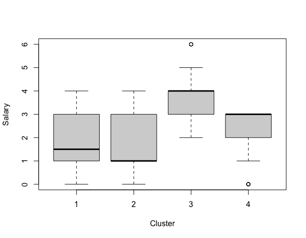
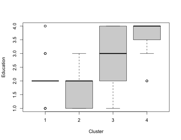
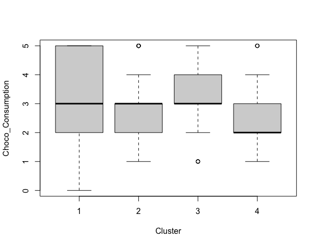
Graph split to 4 groups(Only explained 50.93% of the data), we see that group3 is modestly well-differentiated. 88 customers with higher salary and higher consumption of choco, means more potential to pay at a higher price. Second target is group4, higher educated rate and more sensitive to sustainability, companies can move towards sustainability and attract potential highly educated customers.

1.2 Factor analysis

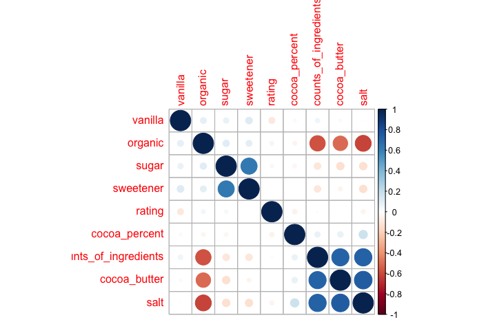
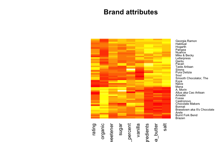
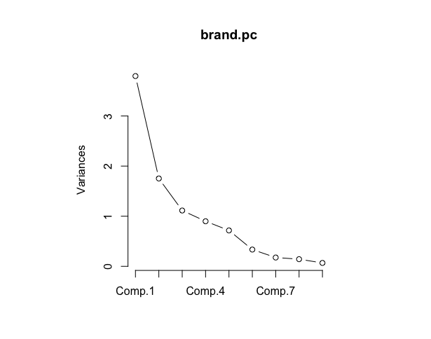
Remove unnecesssary columns from data: product_id,company_location,review_date,country_of_bean_origin,first_taste,second_taste,third_taste. Use heatmap and corrplot to visualizing the relation between factors. Finally using PCA find the position of brand, and looking for future brand positioning.

1.2.1 import and check data

> brand.ratings <- read.csv("2_chocolate_rating.csv", stringsAsFactors = TRUE)
>
> #### remove unnecessary columns
> brand.ratings <- subset(brand.ratings, select = -c(product_id,company_location,review_date,country_of_bean_origin,first_taste,second_taste,third_taste))
> head(brand.ratings)
brand cocoa_percent rating counts_of_ingredients cocoa_butter vanilla organic salt sugar sweetener
1 A. Morin 70 4.00 2 4 8 8 2 9 7
2 A. Morin 70 3.75 1 1 4 7 1 1 1
3 A. Morin 70 3.50 2 3 5 9 2 9 5
4 A. Morin 70 2.75 1 6 10 8 3 4 5
5 A. Morin 70 3.50 1 1 5 8 1 9 9
6 A. Morin 63 3.75 2 8 9 5 3 8 7
> summary(brand.ratings)
brand cocoa_percent rating counts_of_ingredients cocoa_butter vanilla organic salt
Soma : 11 Min. : 60.00 Min. :2.250 Min. : 1.000 Min. : 1.000 Min. : 1.000 Min. : 1.000 Min. : 1.000
Arete : 10 1st Qu.: 70.00 1st Qu.:3.000 1st Qu.: 2.000 1st Qu.: 3.000 1st Qu.: 6.000 1st Qu.: 3.000 1st Qu.: 2.000
Cacao de Origen : 10 Median : 70.00 Median :3.250 Median : 4.000 Median : 6.000 Median : 8.000 Median : 5.000 Median : 5.500
hexx : 8 Mean : 71.53 Mean :3.285 Mean : 5.078 Mean : 5.663 Mean : 7.407 Mean : 5.275 Mean : 5.384
Smooth Chocolator, The: 8 3rd Qu.: 74.00 3rd Qu.:3.500 3rd Qu.: 9.000 3rd Qu.: 8.000 3rd Qu.: 9.000 3rd Qu.: 8.000 3rd Qu.: 9.000
A. Morin : 7 Max. :100.00 Max. :4.000 Max. :10.000 Max. :10.000 Max. :10.000 Max. :10.000 Max. :10.000
(Other) :204
sugar sweetener
Min. : 1.000 Min. : 1.000
1st Qu.: 2.000 1st Qu.: 3.000
Median : 4.000 Median : 4.000
Mean : 4.155 Mean : 4.415
3rd Qu.: 6.000 3rd Qu.: 6.000
Max. :10.000 Max. :10.000

> str(brand.ratings)
'data.frame': 258 obs. of 10 variables:
$ brand : Factor w/ 56 levels "A. Morin","Altus aka Cao Artisan",..: 1 1 1 1 1 1 1 2 2 2 ...
$ cocoa_percent : num 70 70 70 70 70 63 70 60 60 60 ...
$ rating : num 4 3.75 3.5 2.75 3.5 3.75 3.5 3 2.75 2.5 ...
$ counts_of_ingredients: int 2 1 2 1 1 2 1 2 2 3 ...
$ cocoa_butter : int 4 1 3 6 1 8 1 1 1 1 ...
$ vanilla : int 8 4 5 10 5 9 5 7 8 9 ...
$ organic : int 8 7 9 8 8 5 7 5 10 8 ...
$ salt : int 2 1 2 3 1 3 1 2 1 1 ...
$ sugar : int 9 1 9 4 9 8 5 8 7 3 ...
$ sweetener : int 7 1 5 5 9 7 1 7 7 3 ...

1.2.2 Rescaling the data

> brand.sc <- brand.ratings
> brand.sc[,2:10] <- scale (brand.ratings[,2:10])
> head(brand.sc)
brand cocoa_percent rating counts_of_ingredients cocoa_butter vanilla organic salt sugar sweetener
1 A. Morin -0.315311 1.8112654 -0.8883386 -0.5795367 0.2596824 0.96349072 -0.9958673 1.7971812 1.2538261
2 A. Morin -0.315311 1.1780588 -1.1769927 -1.6251343 -1.4919010 0.60989099 -1.2901786 -1.1703244 -1.6561032
3 A. Morin -0.315311 0.5448522 -0.8883386 -0.9280692 -1.0540051 1.31709044 -0.9958673 1.7971812 0.2838497
4 A. Morin -0.315311 -1.3547676 -1.1769927 0.1175284 1.1354741 0.96349072 -0.7015560 -0.0575098 0.2838497
5 A. Morin -0.315311 0.5448522 -1.1769927 -1.6251343 -1.0540051 0.96349072 -1.2901786 1.7971812 2.2238026
6 A. Morin -1.755138 1.1780588 -0.8883386 0.8145935 0.6975783 -0.09730845 -0.7015560 1.4262430 1.2538261
> summary(brand.sc)
brand cocoa_percent rating counts_of_ingredients cocoa_butter vanilla organic
Soma : 11 Min. :-2.3722 Min. :-2.62118 Min. :-1.1770 Min. :-1.6251 Min. :-2.8056 Min. :-1.51171
Arete : 10 1st Qu.:-0.3153 1st Qu.:-0.72156 1st Qu.:-0.8883 1st Qu.:-0.9281 1st Qu.:-0.6161 1st Qu.:-0.80451
Cacao de Origen : 10 Median :-0.3153 Median :-0.08835 Median :-0.3110 Median : 0.1175 Median : 0.2597 Median :-0.09731
hexx : 8 Mean : 0.0000 Mean : 0.00000 Mean : 0.0000 Mean : 0.0000 Mean : 0.0000 Mean : 0.00000
Smooth Chocolator, The: 8 3rd Qu.: 0.5074 3rd Qu.: 0.54485 3rd Qu.: 1.1322 3rd Qu.: 0.8146 3rd Qu.: 0.6976 3rd Qu.: 0.96349
A. Morin : 7 Max. : 5.8554 Max. : 1.81127 Max. : 1.4209 Max. : 1.5117 Max. : 1.1355 Max. : 1.67069
(Other) :204
salt sugar sweetener
Min. :-1.29018 Min. :-1.17032 Min. :-1.6561
1st Qu.:-0.99587 1st Qu.:-0.79939 1st Qu.:-0.6861
Median : 0.03422 Median :-0.05751 Median :-0.2011
Mean : 0.00000 Mean : 0.00000 Mean : 0.0000
3rd Qu.: 1.06431 3rd Qu.: 0.68437 3rd Qu.: 0.7688
Max. : 1.35862 Max. : 2.16812 Max. : 2.7088

> str(brand.sc)
'data.frame': 258 obs. of 10 variables:
$ brand : Factor w/ 56 levels "A. Morin","Altus aka Cao Artisan",..: 1 1 1 1 1 1 1 2 2 2 ...
$ cocoa_percent : num -0.315 -0.315 -0.315 -0.315 -0.315 ...
$ rating : num 1.811 1.178 0.545 -1.355 0.545 ...
$ counts_of_ingredients: num -0.888 -1.177 -0.888 -1.177 -1.177 ...
$ cocoa_butter : num -0.58 -1.625 -0.928 0.118 -1.625 ...
$ vanilla : num 0.26 -1.49 -1.05 1.14 -1.05 ...
$ organic : num 0.963 0.61 1.317 0.963 0.963 ...
$ salt : num -0.996 -1.29 -0.996 -0.702 -1.29 ...
$ sugar : num 1.7972 -1.1703 1.7972 -0.0575 1.7972 ...
$ sweetener : num 1.254 -1.656 0.284 0.284 2.224 ...

> cor(brand.sc[,2:10])
cocoa_percent rating counts_of_ingredients cocoa_butter vanilla organic salt sugar sweetener
cocoa_percent 1.000000000 -0.052546644 0.07123417 0.077370649 -0.02206531 -0.04113143 0.17036000 -0.03957938 0.003483658
rating -0.052546644 1.000000000 0.01437280 0.005272191 -0.09133055 0.04277047 -0.04554864 0.03054233 0.003668166
counts_of_ingredients 0.071234169 0.014372799 1.00000000 0.711183570 0.05157357 -0.57011292 0.72006935 -0.10961457 -0.106926187
cocoa_butter 0.077370649 0.005272191 0.71118357 1.000000000 -0.02054327 -0.50977572 0.74932496 -0.13708717 -0.040725138
vanilla -0.022065307 -0.091330547 0.05157357 -0.020543269 1.00000000 0.08983402 -0.00917223 0.07187530 0.111933243
organic -0.041131426 0.042770467 -0.57011292 -0.509775721 0.08983402 1.00000000 -0.61074144 0.10206892 0.091787605
salt 0.170360004 -0.045548635 0.72006935 0.749324961 -0.00917223 -0.61074144 1.00000000 -0.13863007 -0.134994219
sugar -0.039579384 0.030542330 -0.10961457 -0.137087169 0.07187530 0.10206892 -0.13863007 1.00000000 0.629589888
sweetener 0.003483658 0.003668166 -0.10692619 -0.040725138 0.11193324 0.09178760 -0.13499422 0.62958989 1.000000000

> corrplot(cor(brand.sc[,2:10]), order = "hclust")

organic un-related with countsOfIngredients、cocoaButter and salt salt related with countsOfIngredients and cocoaButter

1.2.3 Mean rating by brand

> brand.mean <- aggregate(. ~ brand, data=brand.sc, mean) 
> brand.mean
brand cocoa_percent rating counts_of_ingredients cocoa_butter vanilla organic salt sugar sweetener
1 A. Morin -0.521000636 0.63531027 -1.05328377 -0.7786981 -0.36588308 0.76143373 -1.03791178 0.84334011 0.283849693
2 Altus aka Cao Artisan -1.857983139 -1.19646594 -0.81617505 -1.6251343 -0.06873946 0.69829093 -1.21660078 0.22069385 0.041355584
3 Ambrosia -0.366733424 0.06994724 -0.88833857 -1.0152024 -0.28768739 1.05189065 -1.14302296 -0.61391709 -0.686126742
4 Amedei -0.109621404 -0.59491968 -0.77287693 -0.6492432 0.34726159 0.96349072 -0.93700505 0.38761604 1.156828484
5 Arete -0.253604135 0.67149350 -1.06153103 -0.9629225 0.25968242 0.68061094 -1.08416070 -0.28007272 -0.007143237
6 Bonnat 0.198913020 1.17805877 -1.03266562 -0.8409361 -0.39716135 1.05189065 -1.06944513 0.03522475 0.162602639
7 Brasstown aka It's Chocolate -0.191897250 0.92477613 -1.11926184 -0.7886562 0.43484076 0.89277077 -0.99586731 0.01667784 0.574842623
8 Brazen -0.315311020 -0.56325935 -1.03266562 -0.8409361 0.04073450 0.52149106 -1.14302296 -0.15024435 -0.443632633
9 Bright -0.041058199 0.12271446 -1.08077463 -1.2766018 -1.34593569 1.31709044 -1.19207484 1.67353512 0.607175171
10 Burnt Fork Bend -0.726690252 -0.51049213 -0.88833857 -0.3471816 -0.76207456 0.84562414 -0.99586731 0.18978233 -0.686126742
11 Cacao de Origen 0.507447444 -0.40495770 -1.06153103 -1.1023355 -0.17821343 1.06957063 -1.14302296 0.16505312 0.332348515
12 Castronovo -0.212466212 0.06994724 -1.17699266 -0.5795367 -0.17821343 1.14029058 -0.99586731 0.31342840 0.283849693
13 Chocolarder -0.109621404 -1.51306923 -1.10482914 -0.3181373 0.58810431 1.22869051 -0.84871166 0.31342840 0.283849693
14 Chocolate Con Amor -0.058199000 -0.56325935 -0.96050209 -0.1438710 0.25968242 0.87509079 -0.84871166 0.68436660 0.041355584
15 Chocolate Makers 1.227361100 0.54485218 -1.03266562 -1.6251343 0.69757827 0.96349072 -1.29017861 -1.17032439 -0.686126742
16 Domori -0.315311020 1.17805877 -0.88833857 -1.2766018 0.47863035 0.60989099 -0.99586731 0.31342840 0.041355584
17 Dormouse 0.850263471 -0.93262986 -1.08077463 -1.2766018 0.40564770 0.37415785 -1.09397107 -0.67574013 -0.201138524
18 Durci -0.315311020 0.75592104 -0.79212054 -0.9861580 -0.03224814 0.96349072 -1.14302296 1.24077389 0.930500649
19 East Van Roasters -0.315311020 0.54485218 -1.08077463 -1.1604242 0.84354355 0.84562414 -1.09397107 0.06613627 0.283849693
20 Fossa 0.044645808 -0.40495770 -0.74401152 -0.9280692 0.36915638 0.87509079 -0.92228948 0.59163205 0.283849693
21 Franceschi -0.109621404 -0.17881249 -1.05328377 -0.8782789 -0.05310033 1.21606195 -1.03791178 0.31342840 0.075997600
22 Fresco -0.178184609 0.22824889 -0.16670333 -0.6957142 0.18669978 -0.27410831 0.03422224 0.37525143 -0.524464002
23 Georgia Ramon 0.370321033 0.12271446 0.84358600 0.6403272 0.69757827 -0.92237447 0.67189673 0.37525143 -0.039475785
24 Habitual 0.164631417 -0.61602657 0.60304092 0.5241497 0.40564770 -0.33304160 0.77000049 0.18978233 0.283849693
25 hexx 0.070357010 -0.87986264 0.41060485 0.2917947 0.09547148 -0.62770803 0.36532246 -0.24297890 0.405096747
26 Hogarth 0.233194623 -0.29942327 0.89169501 0.5822385 0.40564770 -0.21517503 0.42663731 -0.11933283 0.203018324
27 Holy Cacao -0.315311020 0.06994724 0.41060485 0.7274604 0.47863035 -0.71610797 1.13788962 -0.33571345 -0.079891470
28 Johnny Iuzzini 0.219481982 0.41821086 0.84358600 0.2569414 0.60999910 -0.73378795 0.71113823 0.46180368 0.186852050
29 Kto 0.096068212 -0.72156100 0.84358600 0.8145935 0.69757827 -0.59234806 0.59341371 -0.42844799 0.089854406
30 Kyya 0.198913020 -1.14369872 0.55493190 0.5822385 0.69757827 -0.45090817 1.26051933 0.93165873 0.122186954
31 Laia aka Chat-Noir 0.233194623 -0.93262986 0.65114993 0.3498834 0.25968242 -0.92237447 0.86810426 1.05530479 0.768837910
32 Letterpress -0.315311020 0.75592104 -0.11859432 0.4660610 0.69757827 -0.09730845 0.96620803 -0.30480193 0.283849693
33 Mana 0.507447444 -1.77690531 0.26627781 0.1175284 0.11371714 -0.92237447 0.47568919 0.06613627 -0.201138524
34 Map Chocolate -0.521000636 0.33378332 0.50682289 0.2917947 0.25968242 -0.98130776 0.32853354 -0.42844799 0.122186954
35 Maverick -0.315311020 0.06994724 1.06007657 0.9888598 0.47863035 -0.98130776 0.54926702 0.22069385 -0.079891470
36 Mike & Becky -0.315311020 -0.51049213 0.07384175 0.8145935 0.69757827 -0.92237447 0.08327413 -0.18115586 0.283849693
37 Milton -0.315311020 0.86145548 1.42089418 0.4660610 0.47863035 0.07949141 0.32853354 0.68436660 0.041355584
38 Naive 0.198913020 -1.03816429 0.84358600 0.8145935 0.47863035 -0.62770803 1.35862310 -0.42844799 -0.443632633
39 Nibble 0.096068212 -1.35476759 0.77142247 0.7274604 0.25968242 -0.89290783 0.99073397 0.03522475 -0.079891470
40 Nuance -0.315311020 -0.08835441 1.34873066 0.3789278 0.36915638 -1.06970769 0.10780007 -0.24297890 0.405096747
41 Pacari -0.315311020 0.86145548 1.42089418 0.9017266 0.58810431 -0.80450790 0.99073397 0.68436660 -0.201138524
42 Palette de Bine 0.541729047 -0.29942327 0.55493190 0.4079722 0.55161299 -0.39197489 1.06431180 0.49889750 0.688006541
43 Pangea 0.576010649 0.12271446 1.22845812 1.0469485 0.40564770 -0.80450790 0.47568919 -0.18115586 0.122186954
44 Pralus 0.713137060 -0.24665605 0.91574952 0.7274604 0.58810431 -0.36250824 0.40211137 -0.15024435 0.041355584
45 Pump Street Bakery 0.987389881 -0.40495770 -0.02237629 0.8145935 -0.98102248 -0.21517503 0.96620803 -0.42844799 -0.281969894
46 Pura Delizia -0.521000636 0.54485218 -0.59968447 0.4660610 -1.49190097 -0.45090817 0.47568919 -0.24297890 -0.201138524
47 Qantu -0.315311020 0.33378332 -0.11859432 0.9307710 -0.17821343 -0.45090817 1.16241556 -0.42844799 -0.039475785
48 Sirene 1.712200909 0.63531027 0.80234970 0.5158513 -0.67866582 -0.34987968 0.72795602 -0.42844799 -0.478274648
49 Smooth Chocolator, The -0.469578232 0.78230465 0.33844133 0.8145935 -0.94453116 -0.98130776 0.69642267 -0.70665164 -0.504256160
50 Soma -0.090922348 0.89023759 0.44996678 0.5294305 -0.41706571 0.22414584 0.26164461 -0.66449957 -0.730216579
51 Soul 0.198913020 0.22824889 0.77142247 0.6403272 -1.05400512 -0.89290783 1.06431180 -0.52118254 -0.564879687
52 Szanto Tibor -0.315311020 0.38655053 0.84358600 0.2917947 -0.72558324 -0.89290783 0.62284484 -0.89212074 -0.928620850
53 Taste Artisan 0.713137060 0.33378332 1.22845812 0.6984160 0.25968242 0.37415785 0.77000049 -0.79938619 -0.362801263
54 Terroir -0.178184609 0.22824889 0.55493190 0.5822385 -1.49190097 -0.68664132 0.62284484 -0.30480193 -0.766958111
55 Tribar -0.006776596 -0.08835441 -0.02237629 0.2917947 -0.39716135 -0.98130776 1.21146745 -0.42844799 0.041355584
56 Zak's -0.829535060 -0.24665605 1.27656714 1.3373923 -1.05400512 -0.71610797 0.77000049 -0.52118254 -0.443632633
>
> rownames(brand.mean) <- brand.mean[, 1]
> #### Use brand for the row name
> brand.mean <- brand.mean [, -1]
> brand.mean
cocoa_percent rating counts_of_ingredients cocoa_butter vanilla organic salt sugar sweetener
A. Morin -0.521000636 0.63531027 -1.05328377 -0.7786981 -0.36588308 0.76143373 -1.03791178 0.84334011 0.283849693
Altus aka Cao Artisan -1.857983139 -1.19646594 -0.81617505 -1.6251343 -0.06873946 0.69829093 -1.21660078 0.22069385 0.041355584
Ambrosia -0.366733424 0.06994724 -0.88833857 -1.0152024 -0.28768739 1.05189065 -1.14302296 -0.61391709 -0.686126742
Amedei -0.109621404 -0.59491968 -0.77287693 -0.6492432 0.34726159 0.96349072 -0.93700505 0.38761604 1.156828484
Arete -0.253604135 0.67149350 -1.06153103 -0.9629225 0.25968242 0.68061094 -1.08416070 -0.28007272 -0.007143237
Bonnat 0.198913020 1.17805877 -1.03266562 -0.8409361 -0.39716135 1.05189065 -1.06944513 0.03522475 0.162602639
Brasstown aka It's Chocolate -0.191897250 0.92477613 -1.11926184 -0.7886562 0.43484076 0.89277077 -0.99586731 0.01667784 0.574842623
Brazen -0.315311020 -0.56325935 -1.03266562 -0.8409361 0.04073450 0.52149106 -1.14302296 -0.15024435 -0.443632633
Bright -0.041058199 0.12271446 -1.08077463 -1.2766018 -1.34593569 1.31709044 -1.19207484 1.67353512 0.607175171
Burnt Fork Bend -0.726690252 -0.51049213 -0.88833857 -0.3471816 -0.76207456 0.84562414 -0.99586731 0.18978233 -0.686126742
Cacao de Origen 0.507447444 -0.40495770 -1.06153103 -1.1023355 -0.17821343 1.06957063 -1.14302296 0.16505312 0.332348515
Castronovo -0.212466212 0.06994724 -1.17699266 -0.5795367 -0.17821343 1.14029058 -0.99586731 0.31342840 0.283849693
Chocolarder -0.109621404 -1.51306923 -1.10482914 -0.3181373 0.58810431 1.22869051 -0.84871166 0.31342840 0.283849693
Chocolate Con Amor -0.058199000 -0.56325935 -0.96050209 -0.1438710 0.25968242 0.87509079 -0.84871166 0.68436660 0.041355584
Chocolate Makers 1.227361100 0.54485218 -1.03266562 -1.6251343 0.69757827 0.96349072 -1.29017861 -1.17032439 -0.686126742
Domori -0.315311020 1.17805877 -0.88833857 -1.2766018 0.47863035 0.60989099 -0.99586731 0.31342840 0.041355584
Dormouse 0.850263471 -0.93262986 -1.08077463 -1.2766018 0.40564770 0.37415785 -1.09397107 -0.67574013 -0.201138524
Durci -0.315311020 0.75592104 -0.79212054 -0.9861580 -0.03224814 0.96349072 -1.14302296 1.24077389 0.930500649
East Van Roasters -0.315311020 0.54485218 -1.08077463 -1.1604242 0.84354355 0.84562414 -1.09397107 0.06613627 0.283849693
Fossa 0.044645808 -0.40495770 -0.74401152 -0.9280692 0.36915638 0.87509079 -0.92228948 0.59163205 0.283849693
Franceschi -0.109621404 -0.17881249 -1.05328377 -0.8782789 -0.05310033 1.21606195 -1.03791178 0.31342840 0.075997600
Fresco -0.178184609 0.22824889 -0.16670333 -0.6957142 0.18669978 -0.27410831 0.03422224 0.37525143 -0.524464002
Georgia Ramon 0.370321033 0.12271446 0.84358600 0.6403272 0.69757827 -0.92237447 0.67189673 0.37525143 -0.039475785
Habitual 0.164631417 -0.61602657 0.60304092 0.5241497 0.40564770 -0.33304160 0.77000049 0.18978233 0.283849693
hexx 0.070357010 -0.87986264 0.41060485 0.2917947 0.09547148 -0.62770803 0.36532246 -0.24297890 0.405096747
Hogarth 0.233194623 -0.29942327 0.89169501 0.5822385 0.40564770 -0.21517503 0.42663731 -0.11933283 0.203018324
Holy Cacao -0.315311020 0.06994724 0.41060485 0.7274604 0.47863035 -0.71610797 1.13788962 -0.33571345 -0.079891470
Johnny Iuzzini 0.219481982 0.41821086 0.84358600 0.2569414 0.60999910 -0.73378795 0.71113823 0.46180368 0.186852050
Kto 0.096068212 -0.72156100 0.84358600 0.8145935 0.69757827 -0.59234806 0.59341371 -0.42844799 0.089854406
Kyya 0.198913020 -1.14369872 0.55493190 0.5822385 0.69757827 -0.45090817 1.26051933 0.93165873 0.122186954
Laia aka Chat-Noir 0.233194623 -0.93262986 0.65114993 0.3498834 0.25968242 -0.92237447 0.86810426 1.05530479 0.768837910
Letterpress -0.315311020 0.75592104 -0.11859432 0.4660610 0.69757827 -0.09730845 0.96620803 -0.30480193 0.283849693
Mana 0.507447444 -1.77690531 0.26627781 0.1175284 0.11371714 -0.92237447 0.47568919 0.06613627 -0.201138524
Map Chocolate -0.521000636 0.33378332 0.50682289 0.2917947 0.25968242 -0.98130776 0.32853354 -0.42844799 0.122186954
Maverick -0.315311020 0.06994724 1.06007657 0.9888598 0.47863035 -0.98130776 0.54926702 0.22069385 -0.079891470
Mike & Becky -0.315311020 -0.51049213 0.07384175 0.8145935 0.69757827 -0.92237447 0.08327413 -0.18115586 0.283849693
Milton -0.315311020 0.86145548 1.42089418 0.4660610 0.47863035 0.07949141 0.32853354 0.68436660 0.041355584
Naive 0.198913020 -1.03816429 0.84358600 0.8145935 0.47863035 -0.62770803 1.35862310 -0.42844799 -0.443632633
Nibble 0.096068212 -1.35476759 0.77142247 0.7274604 0.25968242 -0.89290783 0.99073397 0.03522475 -0.079891470
Nuance -0.315311020 -0.08835441 1.34873066 0.3789278 0.36915638 -1.06970769 0.10780007 -0.24297890 0.405096747
Pacari -0.315311020 0.86145548 1.42089418 0.9017266 0.58810431 -0.80450790 0.99073397 0.68436660 -0.201138524
Palette de Bine 0.541729047 -0.29942327 0.55493190 0.4079722 0.55161299 -0.39197489 1.06431180 0.49889750 0.688006541
Pangea 0.576010649 0.12271446 1.22845812 1.0469485 0.40564770 -0.80450790 0.47568919 -0.18115586 0.122186954
Pralus 0.713137060 -0.24665605 0.91574952 0.7274604 0.58810431 -0.36250824 0.40211137 -0.15024435 0.041355584
Pump Street Bakery 0.987389881 -0.40495770 -0.02237629 0.8145935 -0.98102248 -0.21517503 0.96620803 -0.42844799 -0.281969894
Pura Delizia -0.521000636 0.54485218 -0.59968447 0.4660610 -1.49190097 -0.45090817 0.47568919 -0.24297890 -0.201138524
Qantu -0.315311020 0.33378332 -0.11859432 0.9307710 -0.17821343 -0.45090817 1.16241556 -0.42844799 -0.039475785
Sirene 1.712200909 0.63531027 0.80234970 0.5158513 -0.67866582 -0.34987968 0.72795602 -0.42844799 -0.478274648
Smooth Chocolator, The -0.469578232 0.78230465 0.33844133 0.8145935 -0.94453116 -0.98130776 0.69642267 -0.70665164 -0.504256160
Soma -0.090922348 0.89023759 0.44996678 0.5294305 -0.41706571 0.22414584 0.26164461 -0.66449957 -0.730216579
Soul 0.198913020 0.22824889 0.77142247 0.6403272 -1.05400512 -0.89290783 1.06431180 -0.52118254 -0.564879687
Szanto Tibor -0.315311020 0.38655053 0.84358600 0.2917947 -0.72558324 -0.89290783 0.62284484 -0.89212074 -0.928620850
Taste Artisan 0.713137060 0.33378332 1.22845812 0.6984160 0.25968242 0.37415785 0.77000049 -0.79938619 -0.362801263
Terroir -0.178184609 0.22824889 0.55493190 0.5822385 -1.49190097 -0.68664132 0.62284484 -0.30480193 -0.766958111
Tribar -0.006776596 -0.08835441 -0.02237629 0.2917947 -0.39716135 -0.98130776 1.21146745 -0.42844799 0.041355584
Zak's -0.829535060 -0.24665605 1.27656714 1.3373923 -1.05400512 -0.71610797 0.77000049 -0.52118254 -0.443632633

> heatmap.2(as.matrix(brand.mean),main = "Brand attributes", trace = "none", key = FALSE, dend = "none"
+ #turn off some options

Some brands related with salt, such as Letterpress、Qantu、Pacari、Kyya、Naive
Some brands related with organic, such as Amedei, Fossa, Castronovo

1.2.4 Principal component analysis (PCA) using princomp()

> brand.pc<- princomp(brand.mean, cor = TRUE)
> #We added "cor =TRUE" to use correlation-based one.
> summary(brand.pc)
Importance of components:
Comp.1 Comp.2 Comp.3 Comp.4 Comp.5 Comp.6 Comp.7 Comp.8 Comp.9
Standard deviation 1.9484877 1.3240155 1.0553760 0.94838484 0.84633623 0.57860956 0.41928231 0.37770849 0.259982952
Proportion of Variance 0.4218449 0.1947797 0.1237576 0.09993709 0.07958722 0.03719878 0.01953307 0.01585152 0.007510126
Cumulative Proportion 0.4218449 0.6166246 0.7403822 0.84031927 0.91990650 0.95710528 0.97663835 0.99248987 1.000000000

> plot(brand.pc,type="l") # scree plot

The elbow occurs at component three. This suggests that the first two components explain most of the variation in the observed brand rating.

> loadings(brand.pc) # pc loadings

Loadings:
Comp.1 Comp.2 Comp.3 Comp.4 Comp.5 Comp.6 Comp.7 Comp.8 Comp.9
cocoa_percent 0.121 0.765 0.271 0.553
rating -0.329 -0.242 0.903
counts_of_ingredients 0.466 0.144 0.133 0.274 -0.149 0.748 -0.283
cocoa_butter 0.477 -0.140 -0.122 -0.595 -0.185 0.579
vanilla 0.502 0.376 0.207 -0.686 0.230 -0.185
organic -0.471 0.131 0.102 -0.778 -0.359
salt 0.484 0.106 0.107 -0.557 -0.649
sugar -0.215 0.482 -0.384 0.416 0.593 -0.151 0.113
sweetener -0.190 0.596 -0.134 0.202 0.137 -0.700 0.183

Comp.1 Comp.2 Comp.3 Comp.4 Comp.5 Comp.6 Comp.7 Comp.8 Comp.9
SS loadings 1.000 1.000 1.000 1.000 1.000 1.000 1.000 1.000 1.000
Proportion Var 0.111 0.111 0.111 0.111 0.111 0.111 0.111 0.111 0.111
Cumulative Var 0.111 0.222 0.333 0.444 0.556 0.667 0.778 0.889 1.000
> brand.pc$scores # the principal components
Comp.1 Comp.2 Comp.3 Comp.4 Comp.5 Comp.6 Comp.7 Comp.8 Comp.9
A. Morin -2.6821054 -0.082708580 -1.40994821 0.570725489 0.49085251 0.18338461 0.117281714 -0.138449624 0.222125496
Altus aka Cao Artisan -2.9741352 -0.051591141 -1.85995919 -2.563339244 -1.66300987 0.13097903 0.303201868 0.526449188 -0.685437305
Ambrosia -1.9137525 -2.368899919 0.43991523 -0.678527355 -0.77889642 0.36199971 -0.253511595 0.148898733 -0.152691868
Amedei -2.5823723 1.971553363 0.06548182 -0.167118353 0.21991151 -1.30388873 -0.375674781 0.417123292 -0.136679953
Arete -2.1702056 -0.945790574 0.23190842 0.654926657 -0.90339862 -0.27205032 0.180399208 -0.080326426 0.100535236
Bonnat -2.4005578 -1.197899532 0.06190293 1.469628715 0.58042613 -0.38552569 -0.087080145 0.039968656 0.074068756
Brasstown aka It's Chocolate -2.5497691 0.133527483 -0.04061230 1.395805810 -0.61251377 -0.84180356 -0.089560874 -0.144162160 0.067272450
Brazen -1.8184009 -1.005611722 0.43555261 -1.230147922 -0.63002787 0.45912632 0.170468440 -0.064477406 0.311590190
Bright -3.7037423 0.414163869 -1.63190725 0.102700490 2.86213684 0.36906420 0.152388138 0.310865000 -0.197363762
Burnt Fork Bend -1.6625728 -1.709402032 -0.88207876 -1.644843428 0.11059053 0.87662539 -0.500865703 -0.110214495 0.338455701
Cacao de Origen -2.5921821 0.055824774 1.09974476 -0.257029615 0.95579544 -0.36550650 0.021096186 0.264035914 -0.075674123
Castronovo -2.5325352 -0.126752242 -0.25831283 -0.004046483 0.33156085 -0.30554860 -0.467607448 -0.168878318 0.136666647
Chocolarder -2.2207668 1.307802587 0.85864663 -1.705624676 -0.19506501 -0.01428509 -0.914520915 -0.321239544 0.159779149
Chocolate Con Amor -1.9007761 0.670491949 0.11709196 -0.620348573 0.29421634 0.61769812 -0.560130738 -0.436771908 0.551468923
Chocolate Makers -1.8579245 -2.204259441 3.65327660 0.944749264 -0.79385429 0.31025351 0.457780690 0.080184237 -0.112091537
Domori -2.4717189 -0.418555050 -0.30112024 1.476626951 -0.84493987 0.44418967 0.556201865 -0.176971531 -0.065225214
Dormouse -1.6163747 -0.573790680 2.78616294 -0.984778126 -0.16073317 -0.22828856 0.696346544 0.154284014 0.109237073
Durci -3.2467009 1.366316064 -1.36938755 1.343686021 0.79119360 -0.14124389 0.102989715 0.247099878 -0.003073146
East Van Roasters -2.6837728 0.239396951 0.28472215 0.845396828 -1.26174552 -0.10762521 0.162505518 -0.184706997 -0.053798374
Fossa -2.3465473 0.884673550 0.38912206 -0.217906869 0.17706864 0.37032870 -0.012113749 0.052158396 -0.059241914
Franceschi -2.5865116 -0.208023319 0.17214188 -0.311579190 0.23054852 0.18080777 -0.351825508 -0.065850200 -0.063028223
Fresco -0.3431384 -0.507481093 -0.23229647 0.070751997 -0.33561536 1.27981256 0.841690012 -0.383017742 -0.156670600
Georgia Ramon 1.6232155 1.150676748 0.26498134 0.776042896 -0.08787525 0.73021028 0.360040767 -0.145401030 0.344721165
Habitual 1.0620088 1.408417040 0.20679968 -0.256329143 0.14603119 -0.09654839 -0.199263082 -0.042347238 -0.204890356
hexx 0.8945803 0.986405829 0.27911766 -0.823341471 0.05290067 -0.91137130 0.215896857 0.391037893 -0.053665334
Hogarth 1.1469231 0.888298143 0.44801300 0.146795869 -0.11225173 -0.17267348 -0.413312452 0.421796760 -0.079016305
Holy Cacao 1.7193074 0.226734338 -0.30964828 0.129600701 -0.98426850 -0.25298514 -0.041078309 -0.590556142 -0.164351653
Johnny Iuzzini 1.1253895 1.247567957 -0.14097718 1.171762685 -0.05453896 0.49259097 0.472104322 -0.020333808 -0.091573476
Kto 1.7272265 0.973823067 0.71344746 -0.485155153 -0.79385313 -0.32876367 -0.322610016 0.219131057 0.094206766
Kyya 1.2196443 2.392140992 0.08609881 -0.785365838 0.47176421 0.99700206 -0.064627360 -0.702134952 -0.261062705
Laia aka Chat-Noir 0.8806390 2.923105952 -0.50273622 -0.361966792 1.15349356 -0.04033924 0.617548018 0.031480014 -0.089609639
Letterpress 0.6051745 0.398736717 -0.33394102 1.207590405 -1.13574976 -0.76005043 -0.322059257 -0.881592716 -0.346321885
Mana 1.2424524 0.909518098 1.17916492 -2.030151126 0.60130333 0.37155938 0.705169097 0.001056193 0.138418715
Map Chocolate 1.1256970 -0.001899391 -0.73005688 0.332513635 -1.15181151 -0.66036279 0.518289540 0.244298956 0.097515381
Maverick 1.8456138 0.805863125 -0.78667732 0.280711960 -0.66679650 0.50954160 0.004065933 0.125501441 0.473074791
Mike & Becky 0.9510565 1.163163024 -0.11474326 -0.450192192 -1.05889582 -0.66072297 0.126707167 -0.134120447 0.814806996
Milton 0.7017978 0.850904718 -1.16300943 1.527503410 -0.35819662 1.14825504 -0.584746995 0.519632202 -0.228518041
Naive 2.4417443 0.319089869 0.92180468 -1.140138484 -0.48419779 0.39789802 -0.287084848 -0.378335636 -0.356746232
Nibble 1.9734880 1.140361527 0.32957158 -1.481479461 0.07908308 0.20080213 0.090557597 -0.062747307 -0.042790815
Nuance 1.4332957 0.986854337 -0.52270722 0.204845388 -0.84737962 -0.60103767 0.416043810 1.168117101 0.091201132
Pacari 1.9470450 0.841192378 -1.30359005 1.428220851 -0.52541881 1.35461573 -0.045551375 -0.117106120 0.063566252
Palette de Bine 0.9298584 2.257452252 0.37466152 0.618514285 0.71206947 -0.35624249 0.067529550 -0.227881300 -0.381700241
Pangea 2.0918919 0.743086202 0.64457687 0.845258973 0.09714474 -0.12746214 -0.154811282 0.523133595 0.462947830
Pralus 1.5025425 0.848741299 1.24672256 0.437250083 0.09124140 0.12844654 -0.313421202 0.312496177 0.232607192
Pump Street Bakery 1.6307924 -1.119099536 1.05475875 -0.464568575 1.97645672 -0.54624494 -0.286472980 -0.427151024 0.025087747
Pura Delizia 0.5045011 -2.031682772 -1.77111102 -0.238237657 0.96235532 -0.92302206 0.202111967 -0.518488381 0.184936862
Qantu 1.4325823 -0.555242055 -0.70143518 0.194149325 -0.26356820 -0.83060181 -0.317473645 -0.896013710 -0.059255689
Sirene 2.0287743 -1.465866212 1.95083466 1.357465166 2.09862837 0.23708772 0.107912320 0.223293081 0.027220665
Smooth Chocolator, The 1.9426612 -2.219944073 -1.28110363 0.197984376 -0.10148814 -0.56237841 0.234920584 -0.116630110 0.250077177
Soma 1.0272560 -2.276609319 -0.13465029 0.682516433 -0.32209432 0.33522067 -0.710966281 0.028455663 -0.046039440
Soul 2.3573617 -1.820518931 -0.34243984 -0.138235420 0.91362197 -0.10331072 0.292826044 0.090846725 -0.195176426
Szanto Tibor 2.1190874 -2.573833100 -0.46454741 -0.315723730 -0.48273243 0.27114066 0.403885143 0.332333083 -0.201129415
Taste Artisan 1.8160636 -0.801618403 1.48053048 0.899555134 -0.11734995 0.13028873 -1.102099959 0.394653864 -0.541862665
Terroir 1.7764533 -2.426405123 -1.13302992 -0.574480808 1.08742023 0.25221874 0.173655136 0.175666615 0.038227332
Tribar 1.5130001 -0.385955737 -0.26682521 -0.265539271 0.26746465 -0.96064380 0.684999665 -0.541489005 -0.348867793
Zak's 2.5174379 -1.426444229 -1.78790183 -1.117084841 -0.02701300 -0.28062025 -0.678142919 0.633397547 0.043738507
>

> biplot(brand.pc, main = "Brand positioning")

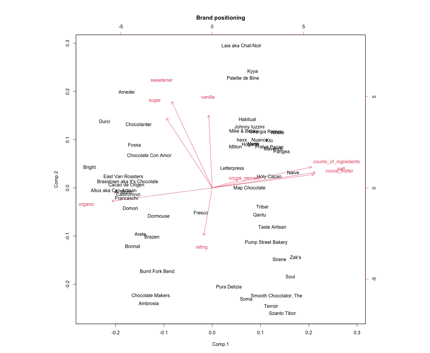
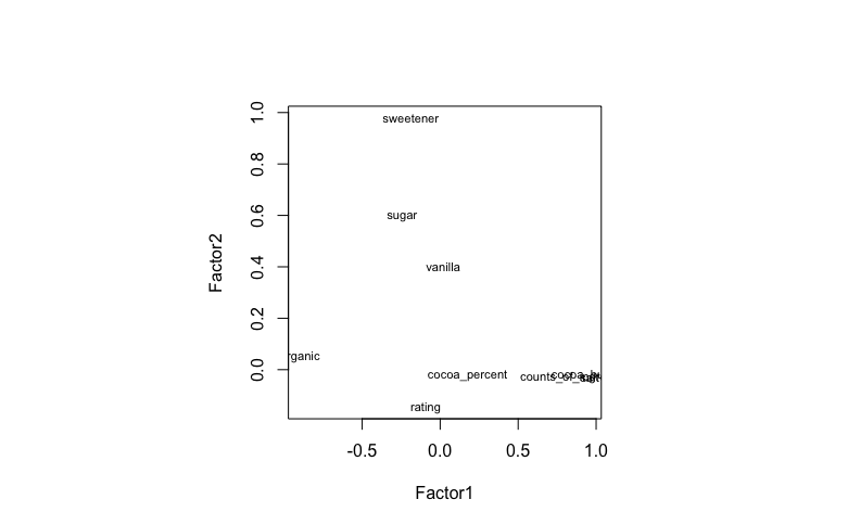
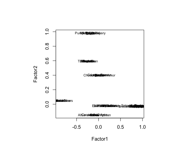
If the brand wants to enhance its differentiation from other brands, brand can focus on balancing the organic and rating aspects. This is more in line with the sustainable development mentioned earlier, and there are fewer brands in this position.

And then, we can use brand.mean or colMeans to calculate the difference distance to target brand.

1.2.5 move forward

Suppose we already have the basis for organic, such as brand Casttronovo. If we want to move forward rating, such as brand Fresco, we should increasing its emphasis on salt, counts_of_ingredients and cocoa_butter. And decrease organic and sweetener.

> colMeans(brand.mean[c("Fresco", "Burnt Fork Bend", "Pura Delizia"), ]) - brand.mean["Castronovo",]
cocoa_percent rating counts_of_ingredients cocoa_butter vanilla organic salt sugar sweetener
Castronovo -0.2628256 0.01758907 0.6254172 0.3872584 -0.5108785 -1.100088 0.833882 -0.2060768 -0.7544261

1.2.6 Factor analysis using factanal() *

> nScree(brand.mean)
noc naf nparallel nkaiser
1 3 1 3 3
> eigen(cor(brand.mean))
eigen() decomposition
$values
[1] 3.79660426 1.75301693 1.11381847 0.89943381 0.71628501 0.33478902 0.17579766 0.14266370 0.06759114

$vectors
[,1] [,2] [,3] [,4] [,5] [,6] [,7] [,8] [,9]
[1,] 0.12098228 -0.05345466 0.76473607 -0.27140650 -0.55335160 -0.042715830 -0.083872256 -0.007471336 -0.09439350
[2,] -0.03942608 0.32895808 -0.24216956 -0.90269635 0.08112631 0.003969369 -0.055740640 0.075143751 -0.03707461
[3,] 0.46644017 -0.14377172 -0.07741629 -0.13320854 0.03448633 -0.274086437 0.149381901 -0.747725837 0.28337944
[4,] 0.47713568 -0.09241339 -0.13970215 -0.02062616 -0.07299798 0.121853132 0.595019898 0.184888897 -0.57918020
[5,] -0.01644575 -0.50210677 0.37649227 -0.20692681 0.68649303 -0.230097021 0.034521520 0.185411405 -0.05715541
[6,] -0.47064300 0.09168746 0.13106717 -0.05057970 -0.07718575 -0.101646053 0.778103705 0.009240990 0.35851266
[7,] 0.48412835 -0.10647051 -0.08160011 -0.02823560 -0.10696045 0.059388537 0.008685290 0.557037340 0.64922598
[8,] -0.21518798 -0.48173066 -0.38411284 -0.08077891 -0.41618156 -0.593141261 -0.082256717 0.151363976 -0.11340603
[9,] -0.19005934 -0.59649010 -0.13377738 -0.20151517 -0.13720262 0.699691310 0.004010208 -0.182634411 0.08836494

> brand.fa <- factanal(brand.mean, factors = 2, rotation = "varimax", scores = "regression")
>
> brand.fl<- brand.fa$loadings[, 1:2]

> plot(brand.fl,type="n") # set up plot
> text(brand.fl,labels=names(brand.mean),cex=.7)
> brand.fs <- brand.fa$scores
> plot(brand.fl,type="n") # set up plot
> text(brand.fl,labels=rownames(brand.mean),cex=.7)

2. Managing Sustainable Competitive Advantage

2.1 Choice-Based Conjoint Analysis

2.1.1 import and check data

> cbc.df <- read.csv("5_conjoint.csv", stringsAsF .... [TRUNCATED] 

> head(cbc.df, n = 5)
Consumer_id Block Choice_id Alternative Choice Origin Manufacture Energy Nuts Tokens Organic Premium Fairtrade Sugar Price
1 1 1 1 1 1 Venezuela Developed Low Nuts only No No Yes Yes High 3
2 1 1 1 2 0 Venezuela UnderDeveloped Low Nuts only Keep & Use No No Yes Low 5
3 1 1 1 3 0 Peru Developing High No Donate Yes No No High 7
4 1 1 2 1 0 Ecuador UnderDeveloped Low Nuts and Fruit Donate Yes No No High 3
5 1 1 2 2 0 Venezuela Developed Low No No No Yes Yes Low 3
Age_Group Gender Salary Education Employment Location_by_region Choco_Consumption Sustainability_Score
1 1 2 1 2 1 1 2 -0.6645
2 1 2 1 2 1 1 2 -0.6645
3 1 2 1 2 1 1 2 -0.6645
4 1 2 1 2 1 1 2 -0.6645
5 1 2 1 2 1 1 2 -0.6645

> summary(cbc.df, digits = 2)
Consumer_id Block Choice_id Alternative Choice Origin Manufacture Energy Nuts
Min. : 1 Min. :1.0 Min. : 1 Min. :1 Min. :0.00 Ecuador :1902 Developed :1418 High:2356 No :2317
1st Qu.: 95 1st Qu.:3.0 1st Qu.: 473 1st Qu.:1 1st Qu.:0.00 Peru :1506 Developing :2311 Low :3314 Nuts and Fruit:1420
Median :190 Median :4.0 Median : 946 Median :2 Median :0.00 Venezuela:2262 UnderDeveloped:1941 Nuts only :1933
Mean :190 Mean :4.5 Mean : 946 Mean :2 Mean :0.33
3rd Qu.:284 3rd Qu.:6.0 3rd Qu.:1418 3rd Qu.:3 3rd Qu.:1.00
Max. :378 Max. :8.0 Max. :1890 Max. :3 Max. :1.00
Tokens Organic Premium Fairtrade Sugar Price Age_Group Gender Salary Education Employment
Donate :1418 No :2664 No :2652 No :2646 High:2670 Min. :2.0 Min. :1.0 Min. :0.0 Min. :0.0 Min. :1.0 Min. : 1.0
Keep & Use:1945 Yes:3006 Yes:3018 Yes:3024 Low :3000 1st Qu.:3.0 1st Qu.:1.0 1st Qu.:1.0 1st Qu.:1.0 1st Qu.:2.0 1st Qu.: 1.0
No :2307 Median :4.0 Median :1.0 Median :2.0 Median :2.0 Median :2.0 Median : 2.0
Mean :4.5 Mean :1.5 Mean :1.6 Mean :2.3 Mean :1.8 Mean : 2.4
3rd Qu.:5.0 3rd Qu.:2.0 3rd Qu.:2.0 3rd Qu.:3.0 3rd Qu.:2.0 3rd Qu.: 3.0
Max. :7.0 Max. :2.0 Max. :2.0 Max. :7.0 Max. :2.0 Max. :10.0
Location_by_region Choco_Consumption Sustainability_Score
Min. :1.0 Min. :1 Min. :-3.26
1st Qu.:1.0 1st Qu.:2 1st Qu.:-0.61
Median :1.0 Median :2 Median : 0.14
Mean :1.2 Mean :2 Mean : 0.00
3rd Qu.:1.0 3rd Qu.:2 3rd Qu.: 0.68
Max. :2.0 Max. :2 Max. : 2.04

> str(cbc.df)
'data.frame': 5670 obs. of 23 variables:
$ Consumer_id : int 1 1 1 1 1 1 1 1 1 1 ...
$ Block : int 1 1 1 1 1 1 1 1 1 1 ...
$ Choice_id : int 1 1 1 2 2 2 3 3 3 4 ...
$ Alternative : int 1 2 3 1 2 3 1 2 3 1 ...
$ Choice : int 1 0 0 0 0 1 0 0 1 0 ...
$ Origin : Factor w/ 3 levels "Ecuador","Peru",..: 3 3 2 1 3 3 1 2 3 1 ...
$ Manufacture : Factor w/ 3 levels "Developed","Developing",..: 1 3 2 3 1 2 1 2 3 2 ...
$ Energy : Factor w/ 2 levels "High","Low": 2 2 1 2 2 1 2 1 2 1 ...
$ Nuts : Factor w/ 3 levels "No","Nuts and Fruit",..: 3 3 1 2 1 2 3 1 2 3 ...
$ Tokens : Factor w/ 3 levels "Donate","Keep & Use",..: 3 2 1 1 3 2 3 2 2 1 ...
$ Organic : Factor w/ 2 levels "No","Yes": 1 1 2 2 1 1 2 2 1 2 ...
$ Premium : Factor w/ 2 levels "No","Yes": 2 1 1 1 2 2 2 1 2 1 ...
$ Fairtrade : Factor w/ 2 levels "No","Yes": 2 2 1 1 2 2 2 1 2 2 ...
$ Sugar : Factor w/ 2 levels "High","Low": 1 2 1 1 2 1 1 2 2 2 ...
$ Price : num 3 5 7 3 3 7 7 4 3 5 ...
$ Age_Group : int 1 1 1 1 1 1 1 1 1 1 ...
$ Gender : int 2 2 2 2 2 2 2 2 2 2 ...
$ Salary : int 1 1 1 1 1 1 1 1 1 1 ...
$ Education : int 2 2 2 2 2 2 2 2 2 2 ...
$ Employment : int 1 1 1 1 1 1 1 1 1 1 ...
$ Location_by_region : int 1 1 1 1 1 1 1 1 1 1 ...
$ Choco_Consumption : int 2 2 2 2 2 2 2 2 2 2 ...
$ Sustainability_Score: num -0.664 -0.664 -0.664 -0.664 -0.664 ...

> cbc.df <- subset(cbc.df, select = -c(Block,Age_Group,Gender,Salary, Education, Employment, Location_by_region, Choco_Consumption, Sustainability_Score))
> head(cbc.df, n = 5)
Consumer_id Choice_id Alternative Choice Origin Manufacture Energy Nuts Tokens Organic Premium Fairtrade Sugar Price
1 1 1 1 1 Venezuela Developed Low Nuts only No No Yes Yes High 3
2 1 1 2 0 Venezuela UnderDeveloped Low Nuts only Keep & Use No No Yes Low 5
3 1 1 3 0 Peru Developing High No Donate Yes No No High 7
4 1 2 1 0 Ecuador UnderDeveloped Low Nuts and Fruit Donate Yes No No High 3
5 1 2 2 0 Venezuela Developed Low No No No Yes Yes Low 3
> summary(cbc.df, digits = 2)
Consumer_id Choice_id Alternative Choice Origin Manufacture Energy Nuts Tokens Organic
Min. : 1 Min. : 1 Min. :1 Min. :0.00 Ecuador :1902 Developed :1418 High:2356 No :2317 Donate :1418 No :2664
1st Qu.: 95 1st Qu.: 473 1st Qu.:1 1st Qu.:0.00 Peru :1506 Developing :2311 Low :3314 Nuts and Fruit:1420 Keep & Use:1945 Yes:3006
Median :190 Median : 946 Median :2 Median :0.00 Venezuela:2262 UnderDeveloped:1941 Nuts only :1933 No :2307
Mean :190 Mean : 946 Mean :2 Mean :0.33
3rd Qu.:284 3rd Qu.:1418 3rd Qu.:3 3rd Qu.:1.00
Max. :378 Max. :1890 Max. :3 Max. :1.00
Premium Fairtrade Sugar Price
No :2652 No :2646 High:2670 Min. :2.0
Yes:3018 Yes:3024 Low :3000 1st Qu.:3.0
Median :4.0
Mean :4.5
3rd Qu.:5.0
Max. :7.0
> str(cbc.df)
'data.frame': 5670 obs. of 14 variables:
$ Consumer_id: int 1 1 1 1 1 1 1 1 1 1 ...
$ Choice_id : int 1 1 1 2 2 2 3 3 3 4 ...
$ Alternative: int 1 2 3 1 2 3 1 2 3 1 ...
$ Choice : int 1 0 0 0 0 1 0 0 1 0 ...
$ Origin : Factor w/ 3 levels "Ecuador","Peru",..: 3 3 2 1 3 3 1 2 3 1 ...
$ Manufacture: Factor w/ 3 levels "Developed","Developing",..: 1 3 2 3 1 2 1 2 3 2 ...
$ Energy : Factor w/ 2 levels "High","Low": 2 2 1 2 2 1 2 1 2 1 ...
$ Nuts : Factor w/ 3 levels "No","Nuts and Fruit",..: 3 3 1 2 1 2 3 1 2 3 ...
$ Tokens : Factor w/ 3 levels "Donate","Keep & Use",..: 3 2 1 1 3 2 3 2 2 1 ...
$ Organic : Factor w/ 2 levels "No","Yes": 1 1 2 2 1 1 2 2 1 2 ...
$ Premium : Factor w/ 2 levels "No","Yes": 2 1 1 1 2 2 2 1 2 1 ...
$ Fairtrade : Factor w/ 2 levels "No","Yes": 2 2 1 1 2 2 2 1 2 2 ...
$ Sugar : Factor w/ 2 levels "High","Low": 1 2 1 1 2 1 1 2 2 2 ...
$ Price : num 3 5 7 3 3 7 7 4 3 5 ...
> xtabs(Choice~Origin, data=cbc.df)
Origin
Ecuador Peru Venezuela
709 495 686

Ecuador(38%) > Venezuela(36%) > Peru(26%)

> xtabs(Choice~Manufacture, data=cbc.df)
Manufacture
Developed Developing UnderDeveloped
436 893 561

Developing > UnderDeveloped > Developed

> xtabs(Choice~Energy, data=cbc.df)
Energy
High Low
922 968

Energy low nearly equals high

> xtabs(Choice~Nuts, data=cbc.df)
Nuts
No Nuts and Fruit Nuts only
568 520 802

Nuts Only(42%) > No(30%) > with Fruit(28%)

> xtabs(Choice~Tokens, data=cbc.df)
Tokens
Donate Keep & Use No
532 740 618

Tokens Keep&Use(39%) > No(32%) > Donate(28%)

> xtabs(Choice~Organic, data=cbc.df)
Organic
No Yes
739 1151

Organic Yes(60%) > No(40%)

> xtabs(Choice~Premium, data=cbc.df)
Premium
No Yes
394 1496

Premium Yes(80%) > No(20%)

> xtabs(Choice~Fairtrade, data=cbc.df)
Fairtrade
No Yes
846 1044

Fairtrade Yes(55%) > No(45%)

> xtabs(Choice~Sugar, data=cbc.df)
Sugar
High Low
1205 685

Sugar High(64%) > Low(36%)

2.1.2 prepare the data

cbc.df$Origin <- relevel(cbc.df$Origin, ref = "Venezuela")
cbc.df$Manufacture <- relevel(cbc.df$Manufacture, ref = "UnderDeveloped")
cbc.df$Energy <- relevel(cbc.df$Energy, ref = "Low")
cbc.df$Nuts <- relevel(cbc.df$Nuts, ref = "No")
cbc.df$Tokens <- relevel(cbc.df$Tokens, ref = "No")
cbc.df$Organic <- relevel(cbc.df$Organic, ref = "No")
cbc.df$Premium <- relevel(cbc.df$Premium, ref = "No")
cbc.df$Fairtrade <- relevel(cbc.df$Fairtrade, ref = "No")
cbc.df$Sugar <- relevel(cbc.df$Sugar, ref = "Low")

2.1.3 Multinomial conjoint model estimation with mlogit()

> cbc.mlogit <- dfidx(cbc.df, choice="Choice",
+ idx=list(c("Choice_id", "Consumer_id"), "Alternative"))
> model<-mlogit(Choice ~ 0+Origin+Manufacture+Energy+Nuts+Tokens+Organic+Premium+Fairtrade+Sugar+Price, data=cbc.mlogit)
> kable(summary(model)$CoefTable)

| | Estimate| Std. Error| z-value| Pr(>&#124;z&#124;)|
|:---------------------|----------:|----------:|----------:|------------------:|
|OriginEcuador | 0.2265894| 0.0836676| 2.7082082| 0.0067648|
|OriginPeru | 0.2194174| 0.0753628| 2.9114832| 0.0035972|
|ManufactureDeveloped | 0.0396353| 0.0812293| 0.4879435| 0.6255898|
|ManufactureDeveloping | -0.2157812| 0.1743582| -1.2375742| 0.2158740|
|EnergyHigh | 0.4153950| 0.1814621| 2.2891551| 0.0220703|
|NutsNuts and Fruit | 0.3435879| 0.0820605| 4.1870067| 0.0000283|
|NutsNuts only | 0.2629300| 0.0751140| 3.5004111| 0.0004645|
|TokensDonate | 0.5203778| 0.0821382| 6.3353922| 0.0000000|
|TokensKeep & Use | 0.1345164| 0.0721562| 1.8642397| 0.0622881|
|OrganicYes | 0.3947520| 0.0614207| 6.4270217| 0.0000000|
|PremiumYes | 1.3982032| 0.0666952| 20.9640710| 0.0000000|
|FairtradeYes | 0.4648390| 0.0613058| 7.5822972| 0.0000000|
|SugarHigh | 0.6121655| 0.0632706| 9.6753519| 0.0000000|
|Price | -0.0824375| 0.0207685| -3.9693491| 0.0000721|

Demonstrated that positive value of utility means prefer than reference value, meanwhile negative value indicates that they prefer reference level.
In case of the Nuts attribute, customers prefer more nuts, etc.

2.1.4 Model fit

> model.constraint <-mlogit(Choice ~ 0+Nuts, data = cbc.mlogit)
> lrtest(model, model.constraint)
Likelihood ratio test

Model 1: Choice ~ 0 + Origin + Manufacture + Energy + Nuts + Tokens +
Organic + Premium + Fairtrade + Sugar + Price
Model 2: Choice ~ 0 + Nuts
#Df LogLik Df Chisq Pr(>Chisq)
1 14 -1566.0
2 2 -2021.2 -12 910.45 < 2.2e-16 ***
---
Signif. codes: 0 ‘***’ 0.001 ‘**’ 0.01 ‘*’ 0.05 ‘.’ 0.1 ‘ ’ 1

Means the larger model (our first model) fits the data better. So, we should keep all the variables.

2.1.5 Interpreting Conjoint Analysis Findings

According to mlogit() results, customers prefer:

  1. Higher energy
  2. More Nuts
  3. Donate loyalty points with chocolates
  4. Be Organic
  5. Farmers paid a premium price
  6. Faire trade certified
  7. Higher sugar
  8. Lower price
  9. Origin Ecuador or Peru
  10. Developed Manufacture

We test the prediction for the first six choice sets in the data.

> kable(head(predict(model,cbc.mlogit)))


| 1| 2| 3|
|---------:|---------:|---------:|
| 0.6954121| 0.0868465| 0.2177414|
| 0.2571232| 0.2116132| 0.5312636|
| 0.6276737| 0.0693051| 0.3030212|
| 0.3751338| 0.3188902| 0.3059760|
| 0.2320737| 0.6858870| 0.0820393|
| 0.6530199| 0.2196068| 0.1273733|

We can see that, in group 2, choice 3 is more prefered, which means customers may pay more for higher energy and higher nuts and fruit.

And then, Measure the accuracy of prediction across all data:

> predicted_alternative <- apply(predict(model,cbc.mlogit),1,which.max) 
> selected_alternative <- cbc.mlogit$Alternative[cbc.mlogit$Choice>0]
> confusionMatrix(table(predicted_alternative,selected_alternative),positive = "1")
Confusion Matrix and Statistics

selected_alternative
predicted_alternative 1 2 3
1 315 104 102
2 142 705 140
3 102 61 219

Overall Statistics

Accuracy : 0.6556
95% CI : (0.6336, 0.677)
No Information Rate : 0.4603
P-Value [Acc > NIR] : < 2.2e-16

Kappa : 0.4522

Mcnemar's Test P-Value : 4.785e-08

Statistics by Class:

Class: 1 Class: 2 Class: 3
Sensitivity 0.5635 0.8103 0.4751
Specificity 0.8452 0.7235 0.8859
Pos Pred Value 0.6046 0.7143 0.5733
Neg Pred Value 0.8218 0.8173 0.8395
Prevalence 0.2958 0.4603 0.2439
Detection Rate 0.1667 0.3730 0.1159
Detection Prevalence 0.2757 0.5222 0.2021
Balanced Accuracy 0.7044 0.7669 0.6805

If the predictions were random, the accuracy would be 33.3% (for three alternatives). Our simple model is doing much better than that – although it is not perfect.

2.2 Willingness to pay

2.2.1 What is the Nuts’ value

> (coef(model)["NutsNuts and Fruit"]-coef(model)["NutsNuts only"]) / (-coef(model)["Price"])
NutsNuts and Fruit
0.9784127

The dollar value of an upgrade from Nuts only to Nuts and Fruit.

2.2.2 Willingness to Pay for an Attribute Upgrade

> coef(model)["NutsNuts and Fruit"] / (-coef(model)["Price"])
NutsNuts and Fruit
4.167859

The dollar value of an upgrade from No Nuts to Nuts and Fruit (No Nuts is reference level. Hence its coeff is 0)

> coef(model)["EnergyHigh"] / (-coef(model)["Price"])
EnergyHigh
5.038907

The dollar value of an upgrade from Energy Low to Energy High (Energy Low is reference level. Hence its coeff is 0)

2.3 Market Basket

2.3.1 Retail Transaction Data: Groceries

> retail.raw <- readLines("6_groceries.dat")

> head(retail.raw)
[1] "fruit, semi-finished bread, margarine, ready soups" "crisps and nuts, yogurt, coffee"
[3] "whole milk" "pip fruit, yogurt, cream cheese, meat spreads"
[5] "milk chocolate, whole milk, condensed milk, dark chocolate" "whole milk, butter, yogurt, rice, abrasive cleaner"

> tail(retail.raw)
[1] "crisps and nuts, milk chocolate, domestic eggs, zwieback, ketchup, soda, dishes"
[2] "sausage, chicken, sweet, hamburger meat, fruit, grapes, biscuits and crackers, whole milk, butter, whipped/sour cream, flour, coffee, red/blush wine, salty snack, milk chocolate, hygiene articles, napkins"
[3] "cooking milk chocolate"
[4] "chicken, fruit, milk chocolate, butter, yogurt, frozen dessert, domestic eggs, bread, rum, cling film/bags"
[5] "semi-finished bread, bottled water, soda, bottled beer"
[6] "chicken, crisps and nuts, milk chocolate, vinegar, shopping bags"

> summary(retail.raw)
Length Class Mode
9835 character character

> retail.list <- strsplit(retail.raw, ",")
> names(retail.list) <- paste("Trans", 1:length(retail.list))
> str(retail.list)
List of 9835
$ Trans 1 : chr [1:4] "fruit" " semi-finished bread" " margarine" " ready soups"
$ Trans 2 : chr [1:3] "crisps and nuts" " yogurt" " coffee"
$ Trans 3 : chr "whole milk"
$ Trans 4 : chr [1:4] "pip fruit" " yogurt" " cream cheese" " meat spreads"
$ Trans 5 : chr [1:4] "milk chocolate" " whole milk" " condensed milk" " dark chocolate"
$ Trans 6 : chr [1:5] "whole milk" " butter" " yogurt" " rice" ...
$ Trans 7 : chr "bread"
$ Trans 8 : chr [1:5] "milk chocolate" " UHT-milk" " bread" " bottled beer" ...
$ Trans 9 : chr "potted plants"
$ Trans 10 : chr [1:2] "whole milk" " cereals"
$ Trans 11 : chr [1:5] "crisps and nuts" " milk chocolate" " white bread" " bottled water" ...
$ Trans 12 : chr [1:9] "fruit" " crisps and nuts" " whole milk" " butter" ...
$ Trans 13 : chr "sweet"
$ Trans 14 : chr [1:3] "frankfurter" " bread" " soda"
$ Trans 15 : chr [1:2] "chicken" " crisps and nuts"
$ Trans 16 : chr [1:4] "butter" " sugar" " fruit/vegetable juice" " newspapers"
$ Trans 17 : chr "fruit/vegetable juice"
$ Trans 18 : chr "packaged fruit/vegetables"
$ Trans 19 : chr "milk chocolate"
$ Trans 20 : chr "specialty bar"
$ Trans 21 : chr "milk chocolate"
$ Trans 22 : chr [1:2] "butter milk" " pastry"
$ Trans 23 : chr "whole milk"
$ Trans 24 : chr [1:5] "crisps and nuts" " cream cheese" " processed cheese" " detergent" ...
$ Trans 25 : chr [1:11] "crisps and nuts" " biscuits and crackers" " milk chocolate" " frozen dessert" ...
$ Trans 26 : chr [1:2] "bottled water" " canned beer"
$ Trans 27 : chr "yogurt"
$ Trans 28 : chr [1:4] "sausage" " bread" " soda" " milk chocolate"
$ Trans 29 : chr "milk chocolate"
$ Trans 30 : chr [1:6] "brown bread" " soda" " fruit/vegetable juice" " canned beer" ...
$ Trans 31 : chr [1:4] "yogurt" " beverages" " bottled water" " specialty bar"
$ Trans 32 : chr [1:7] "hamburger meat" " milk chocolate" " bread" " spices" ...
$ Trans 33 : chr [1:5] "biscuits and crackers" " milk chocolate" " whole milk" " beverages" ...
$ Trans 34 : chr [1:8] "beef" " berries" " milk chocolate" " whole milk" ...
$ Trans 35 : chr [1:3] "sweet" " grapes" " detergent"
$ Trans 36 : chr [1:2] "pastry" " soda"
$ Trans 37 : chr "fruit/vegetable juice"
$ Trans 38 : chr "canned beer"
$ Trans 39 : chr [1:4] "biscuits and crackers" " milk chocolate" " whole milk" " dessert"
$ Trans 40 : chr [1:3] "fruit" " zwieback" " newspapers"
$ Trans 41 : chr [1:6] "sausage" " bread" " soda" " canned beer" ...
$ Trans 42 : chr [1:13] "crisps and nuts" " biscuits and crackers" " whole milk" " yogurt" ...
$ Trans 43 : chr [1:2] "berries" " yogurt"
$ Trans 44 : chr "canned beer"
$ Trans 45 : chr [1:8] "butter milk" " yogurt" " cream cheese" " spread cheese" ...
$ Trans 46 : chr "coffee"
$ Trans 47 : chr [1:2] "pastry" " bottled water"
$ Trans 48 : chr "bread"
$ Trans 49 : chr "misc. beverages"
$ Trans 50 : chr [1:10] "biscuits and crackers" " milk chocolate" " butter" " curd" ...
$ Trans 51 : chr [1:4] "sausage" " bread" " cat food" " newspapers"
$ Trans 52 : chr "canned beer"
$ Trans 53 : chr [1:4] "ham" " grapes" " milk chocolate" " whole milk"
$ Trans 54 : chr [1:10] "turkey" " crisps and nuts" " milk chocolate" " curd" ...
$ Trans 55 : chr [1:5] "whole milk" " yogurt" " processed cheese" " pickled vegetables" ...
$ Trans 56 : chr [1:4] "whole milk" " curd" " yogurt" " pastry"
$ Trans 57 : chr [1:3] "packaged fruit/vegetables" " brown bread" " canned beer"
$ Trans 58 : chr [1:7] "bread" " oil" " bottled water" " chewing gum" ...
$ Trans 59 : chr [1:6] "ham" " sweet" " whipped/sour cream" " ice cream" ...
$ Trans 60 : chr [1:3] "bread" " pastry" " sugar"
$ Trans 61 : chr [1:7] "milk chocolate" " whole milk" " frozen vegetables" " canned fish" ...
$ Trans 62 : chr [1:2] "sausage" " pastry"
$ Trans 63 : chr [1:3] "sausage" " sweet" " whole milk"
$ Trans 64 : chr [1:5] "frankfurter" " crisps and nuts" " bread" " brown bread" ...
$ Trans 65 : chr [1:3] "bread" " pastry" " soda"
$ Trans 66 : chr "whole milk"
$ Trans 67 : chr [1:2] "curd cheese" " coffee"
$ Trans 68 : chr [1:2] "red/blush wine" " newspapers"
$ Trans 69 : chr [1:3] "sausage" " whole milk" " curd"
$ Trans 70 : chr [1:8] "crisps and nuts" " pip fruit" " berries" " whole milk" ...
$ Trans 71 : chr "red/blush wine"
$ Trans 72 : chr [1:7] "whole milk" " butter" " margarine" " specialty fat" ...
$ Trans 73 : chr [1:8] "frankfurter" " fruit" " whole milk" " domestic eggs" ...
$ Trans 74 : chr [1:3] "whole milk" " meat spreads" " soda"
$ Trans 75 : chr "frozen potato products"
$ Trans 76 : chr [1:4] "milk chocolate" " whole milk" " bread" " sugar"
$ Trans 77 : chr [1:5] "fruit" " whole milk" " curd" " butter milk" ...
$ Trans 78 : chr [1:5] "flour" " salt" " bottled water" " fruit/vegetable juice" ...
$ Trans 79 : chr [1:4] "sugar" " bottled water" " soda" " bottled beer"
$ Trans 80 : chr [1:2] "frozen meals" " coffee"
$ Trans 81 : chr "milk chocolate"
$ Trans 82 : chr [1:10] "biscuits and crackers" " whole milk" " frozen vegetables" " domestic eggs" ...
$ Trans 83 : chr [1:4] "biscuits and crackers" " onions" " hard cheese" " frozen vegetables"
$ Trans 84 : chr [1:7] "herbs" " condensed milk" " frozen vegetables" " salt" ...
$ Trans 85 : chr "bottled water"
$ Trans 86 : chr [1:7] "sausage" " biscuits and crackers" " onions" " yogurt" ...
$ Trans 87 : chr [1:2] "coffee" " newspapers"
$ Trans 88 : chr [1:3] "beef" " milk chocolate" " whipped/sour cream"
$ Trans 89 : chr [1:2] "berries" " yogurt"
$ Trans 90 : chr "soda"
$ Trans 91 : chr "berries"
$ Trans 92 : chr [1:3] "fruit/vegetable juice" " salty snack" " candles"
$ Trans 93 : chr [1:4] "fruit" " butter milk" " yogurt" " cream cheese"
$ Trans 94 : chr [1:9] "beef" " hamburger meat" " fruit" " berries" ...
$ Trans 95 : chr "detergent"
$ Trans 96 : chr [1:2] "grapes" " photo/film"
$ Trans 97 : chr [1:9] "sausage" " sliced cheese" " bread" " brown bread" ...
$ Trans 98 : chr [1:10] "chicken" " hamburger meat" " fruit" " crisps and nuts" ...
$ Trans 99 : chr [1:3] "whole milk" " yogurt" " brown bread"
[list output truncated]
>
> some(retail.list) #note: random sample; your results may vary
$`Trans 918`
[1] "beef" " fruit" " UHT-milk" " brown bread" " soda" " bottled beer"
[7] " canned beer" " dark chocolate"

$`Trans 1371`
[1] "bottled beer"

$`Trans 1563`
[1] "bread"

$`Trans 2440`
[1] "shopping bags"

$`Trans 3235`
[1] "bottled water" " bottled beer"

$`Trans 3260`
[1] "frankfurter" " milk chocolate" " whole milk" " spread cheese"
[5] " sugar" " soda" " bottled beer" " house keeping products"

$`Trans 8306`
[1] "beef" " sweet" " grapes" " berries"
[5] " biscuits and crackers" " milk chocolate" " packaged fruit/vegetables" " yogurt"
[9] " newspapers"

$`Trans 9069`
[1] "berries" " biscuits and crackers" " whipped/sour cream" " soda"

$`Trans 9315`
[1] "whole milk"

$`Trans 9404`
[1] "sausage" " bottled water" " canned beer" " hygiene articles" " shopping bags"

> retail.trans <- as(retail.list, "transactions") #takes a few seconds
Warning message:
In asMethod(object) : removing duplicated items in transactions
> summary(retail.trans)
transactions as itemMatrix in sparse format with
9835 rows (elements/itemsets/transactions) and
324 columns (items) and a density of 0.01357711

most frequent items:
whole milk milk chocolate bread soda yogurt (Other)
1796 1782 1473 1421 1147 35645

element (itemset/transaction) length distribution:
sizes
1 2 3 4 5 6 7 8 9 10 11 12 13 14 15 16 17 18 19 20 21 22 23 24 25
2159 1643 1301 1007 854 649 553 433 346 250 178 116 80 73 56 46 27 13 16 10 9 4 4 1 1
27 28 29 32
1 3 1 1

Min. 1st Qu. Median Mean 3rd Qu. Max.
1.000 2.000 3.000 4.399 6.000 32.000

includes extended item information - examples:
labels
1 abrasive cleaner
2 artif. sweetener
3 baby cosmetics

includes extended transaction information - examples:
transactionID
1 Trans 1
2 Trans 2
3 Trans 3

Looking at the summary() of the resulting object, we see that the transaction-by-item matrix is 9,835 rows by 324 columns. Of those 3.1 million intersections, only 1% have positive data (density) because most items are not purchased in most transactions. Item whole milk appears the most frequently and occurs in 1,796 baskets of all transactions. 2,159 of the transactions contain only a single item (“sizes” = 1) and the median basket size is 3 items.

2.3.2 Retail Transaction Data: Groceries

We now use apriori(data, parameters = …) to find association rules with the apriori algorithm. At a conceptual level, the apriori algorithm searches through the item sets that frequently occur in a list of transactions. For each item set, it evaluates the various possible rules that express associations among the items at or above a particular level of support, and then retains the rules that show confidence above some threshold value. To control the extent that apriori() searches, we use the parameter=list() control to instruct the algorithm to search rules that have a minimum support of 0.01 (1% transactions) and extract the ones that further demonstrate a minimum confidence of 0.3. The resulting rules set is assigned to the groc.rules object:

> inspect(head(retail.trans,3))
items transactionID
[1] { margarine, ready soups, semi-finished bread, fruit} Trans 1
[2] { coffee, yogurt, crisps and nuts} Trans 2
[3] {whole milk} Trans 3
> # Finding rules
> groc.rules <- apriori(retail.trans, parameter = list(supp=0.01, conf=0.3, target="rules"))
Apriori

Parameter specification:
confidence minval smax arem aval originalSupport maxtime support minlen maxlen target ext
0.3 0.1 1 none FALSE TRUE 5 0.01 1 10 rules TRUE

Algorithmic control:
filter tree heap memopt load sort verbose
0.1 TRUE TRUE FALSE TRUE 2 TRUE

Absolute minimum support count: 98

set item appearances ...[0 item(s)] done [0.00s].
set transactions ...[324 item(s), 9835 transaction(s)] done [0.01s].
sorting and recoding items ... [97 item(s)] done [0.00s].
creating transaction tree ... done [0.01s].
checking subsets of size 1 2 3 4 done [0.00s].
writing ... [118 rule(s)] done [0.00s].
creating S4 object ... done [0.00s].
  • “sorting and recoding items … [97 item(s)] done [0.00s].”: tells us that the rules found are using 97 of the total number of items. If this number is too small (only a tiny set of your items) or too large (almost all of them), then you might wish to adjust the support and confidence levels.

  • “writing … [118 rule(s)] done [0.00s].”: Next, check the number of rules found, as indicated on the “writing …” line. In this case, the algorithm found 118 rules. If this number is too low, it suggests the need to lower the support or confidence levels; if it is too high (such as many more rules than items), you might increase the support or confidence levels.

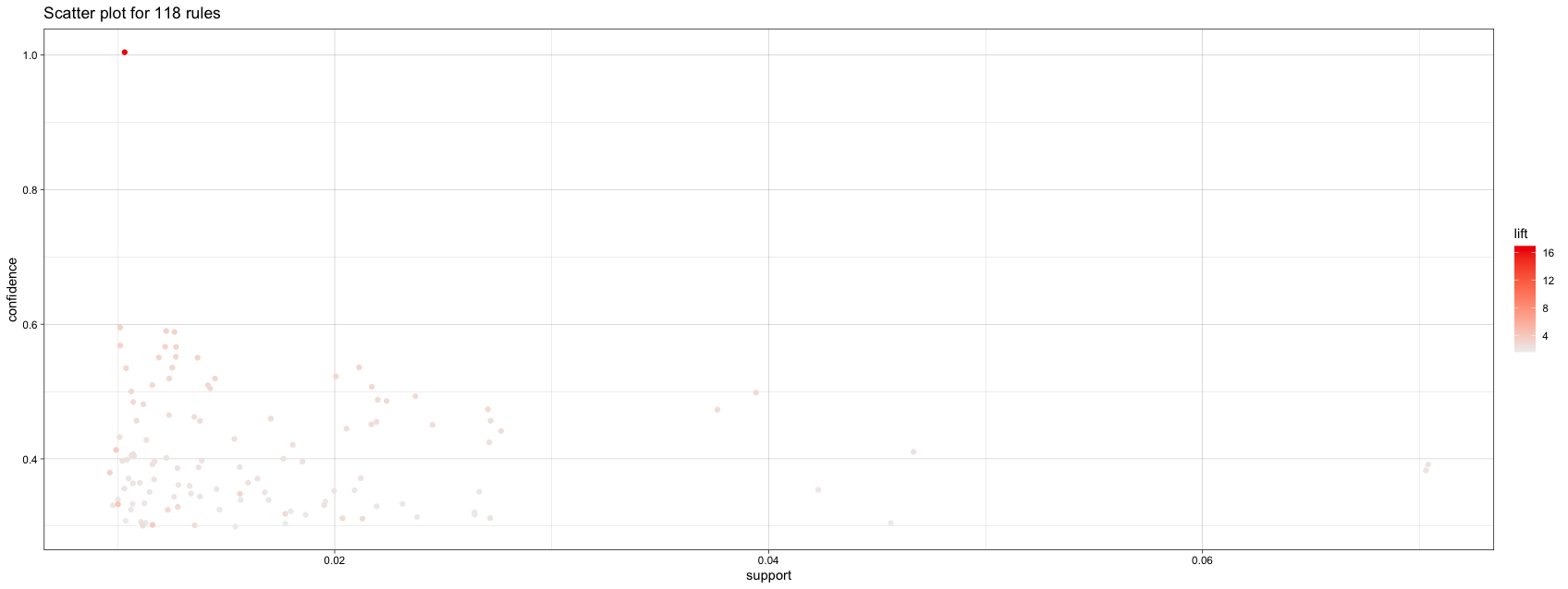
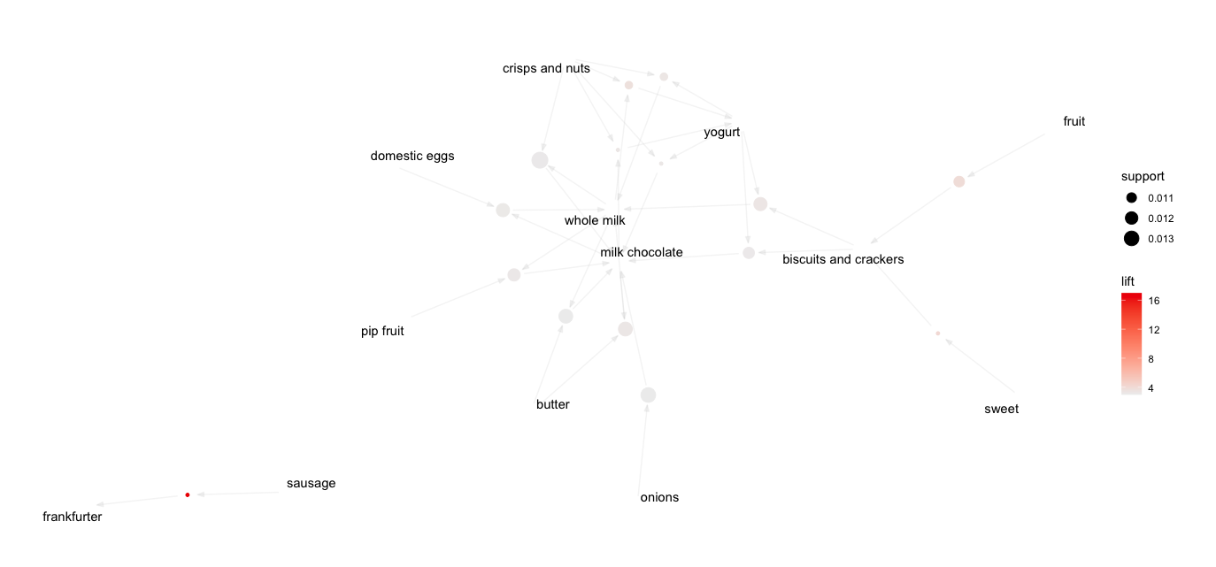
Once we have a rule set from apriori(), we use inspect(rules) to examine the association rules. The complete list of 118 from above is too long to examine here, so we select a subset of them with high lift, lift > 3. We find that five of the rules in our set have lift greater than 3.0:

> inspect(subset(groc.rules, lift > 3))
lhs rhs support confidence coverage lift count
[1] { sausage} => {frankfurter} 0.01006609 1.0000000 0.01006609 16.956897 99
[2] {sweet} => { biscuits and crackers} 0.01006609 0.3256579 0.03091002 4.085262 99
[3] { onions} => { milk chocolate} 0.01301474 0.5446809 0.02389426 3.006137 128
[4] { fruit} => { biscuits and crackers} 0.01128622 0.3074792 0.03670564 3.857217 111
[5] { butter, milk chocolate} => { whole milk} 0.01260803 0.5876777 0.02145399 3.218157 124
[6] { pip fruit, whole milk} => { milk chocolate} 0.01189629 0.5652174 0.02104728 3.119480 117
[7] { domestic eggs, milk chocolate} => { whole milk} 0.01230300 0.5654206 0.02175902 3.096276 121
[8] { crisps and nuts, yogurt} => { whole milk} 0.01047280 0.5953757 0.01759024 3.260312 103
[9] { crisps and nuts, whole milk} => { yogurt} 0.01047280 0.4186992 0.02501271 3.590154 103
[10] { crisps and nuts, yogurt} => { milk chocolate} 0.01006609 0.5722543 0.01759024 3.158317 99
[11] { crisps and nuts, milk chocolate} => { yogurt} 0.01006609 0.3750000 0.02684291 3.215453 99
[12] { crisps and nuts, whole milk} => { milk chocolate} 0.01372649 0.5487805 0.02501271 3.028763 135
[13] { biscuits and crackers, yogurt} => { whole milk} 0.01230300 0.5960591 0.02064057 3.264054 121
[14] { biscuits and crackers, yogurt} => { milk chocolate} 0.01148958 0.5566502 0.02064057 3.072197 113

The first rule tells us that if a transaction contains {sausage} then it is also relatively more likely to contain {frankfurter}. The support shows that the combination appears in 1% of baskets, and the lift shows that the combination is 17× more likely to occur together than one would expect from the individual rates of incidence alone.

A store might form several insights on the basis of such information. For instance, the store might create a display for frankfurter near the sausage to encourage shoppers who are examining sausage to purchase those frankfurter with them. It might also suggest putting coupons for frankfurter in the sausage area or featuring recipe cards somewhere in the store.

plot(groc.rules)

In that chart, we see that most rules involve item combinations that infrequently occur (that is, they have low support) while confidence is relatively smoothly distributed.

Simply showing points is not very useful, and a key feature with arulesViz is interactive plotting. In the above figure, there are some rules on the upper left with a high lift. We can use interactive plotting to inspect those rules. To do this, add interactive=TRUE to the plot() command:

plot(groc.rules, engine = "plotly", interactive=TRUE)

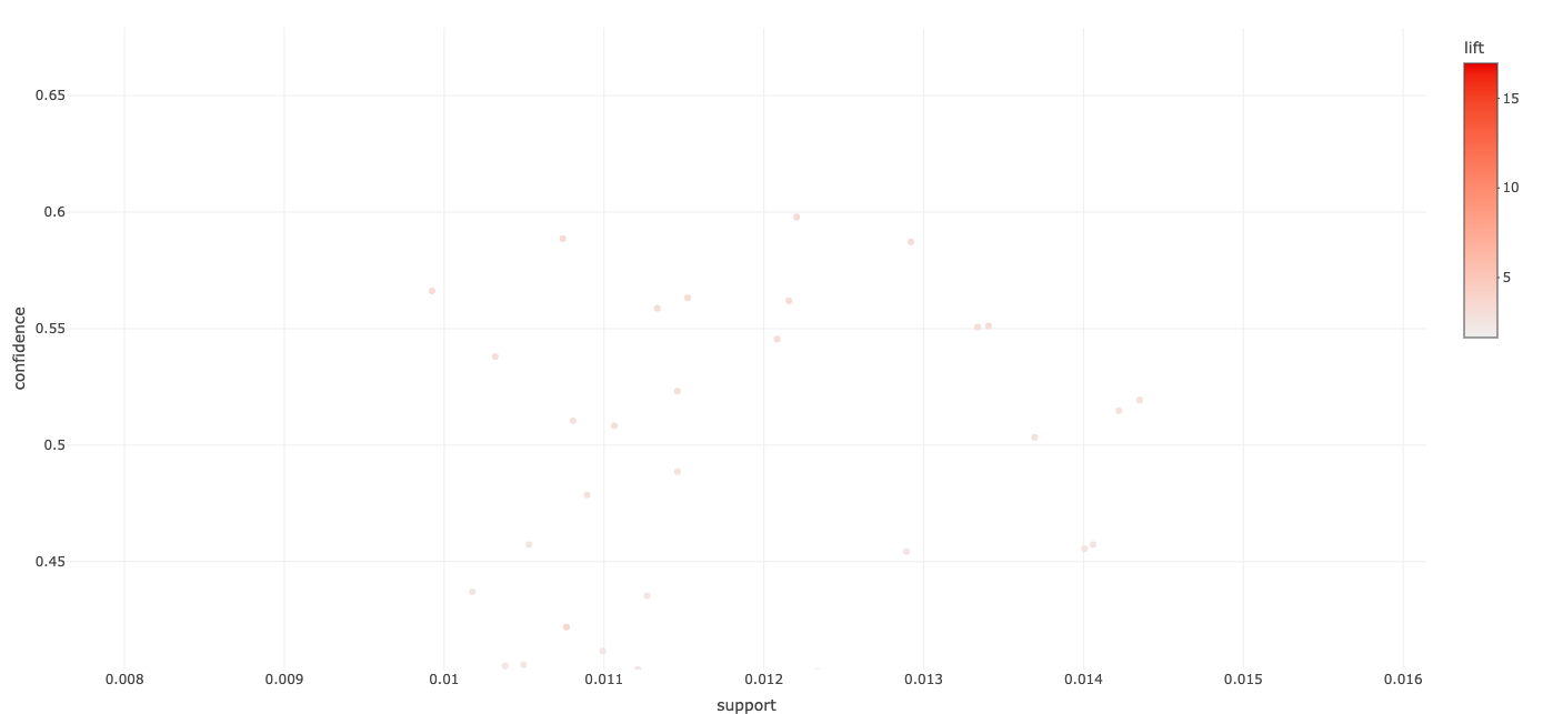
One rule tells us that the combination {crisps and nuts, yogurt} occurs in about 1.0 % of baskets (support=0.0105), and when it occurs, it highly likely includes {whole milk} (confidence= 0.595). The combination occurs 3 times more often than we would expect from the individual incidence rates of {crisps and nuts, yogurt} and {whole milk} considered separately (lift=3.26).

A common goal in market basket analysis is to find rules with high lift. We can find such rules easily by sorting the larger set of rules by lift. We extract the 15 rules with the highest lift using sort() to order the rules by lift and to take 50 from the head():

> # Finding and Plotting Subsets of Rules
> groc.hi <- head(sort(groc.rules, by="lift"), 15)
> inspect(groc.hi)
lhs rhs support confidence coverage lift count
[1] { sausage} => {frankfurter} 0.01006609 1.0000000 0.01006609 16.956897 99
[2] {sweet} => { biscuits and crackers} 0.01006609 0.3256579 0.03091002 4.085262 99
[3] { fruit} => { biscuits and crackers} 0.01128622 0.3074792 0.03670564 3.857217 111
[4] { crisps and nuts, whole milk} => { yogurt} 0.01047280 0.4186992 0.02501271 3.590154 103
[5] { biscuits and crackers, yogurt} => { whole milk} 0.01230300 0.5960591 0.02064057 3.264054 121
[6] { crisps and nuts, yogurt} => { whole milk} 0.01047280 0.5953757 0.01759024 3.260312 103
[7] { butter, milk chocolate} => { whole milk} 0.01260803 0.5876777 0.02145399 3.218157 124
[8] { crisps and nuts, milk chocolate} => { yogurt} 0.01006609 0.3750000 0.02684291 3.215453 99
[9] { crisps and nuts, yogurt} => { milk chocolate} 0.01006609 0.5722543 0.01759024 3.158317 99
[10] { pip fruit, whole milk} => { milk chocolate} 0.01189629 0.5652174 0.02104728 3.119480 117
[11] { domestic eggs, milk chocolate} => { whole milk} 0.01230300 0.5654206 0.02175902 3.096276 121
[12] { biscuits and crackers, yogurt} => { milk chocolate} 0.01148958 0.5566502 0.02064057 3.072197 113
[13] { crisps and nuts, whole milk} => { milk chocolate} 0.01372649 0.5487805 0.02501271 3.028763 135
[14] { onions} => { milk chocolate} 0.01301474 0.5446809 0.02389426 3.006137 128
[15] { butter, whole milk} => { milk chocolate} 0.01260803 0.5414847 0.02328419 2.988497 124

Support and lift are identical for an item set regardless of the items’ order within a rule (left-hand or right- hand side of the rule). However, confidence reflects direction because it computes the occurrence of the right-hand set conditional on the left-hand side set.
A graph display of rules may be useful to seek themes and patterns at a higher level. We chart the top 15 rules byliftwithplot(… ,method=“graph”):

The positioning of items on the resulting graph may differ for your system, but the item clusters should be similar. Each circle represents a rule, with inbound arrows coming from items on the left-hand side of the rule and outbound arrows going to the right-hand side. The size (area) of the circle represents the rule’s support, and shade represents lift (darker indicates higher lift).

3 Managing Resources Trade-offs

3.1 Selecting Advertising platforms

3.1.1 import and check data

spending.data <- read.csv("7_advertising.csv")
str(spending.data)
plot(spending.data$radio, spending.data$sales)
plot(spending.data$magazines, spending.data$sales)
plot(spending.data$social_media, spending.data$sales)
plot(spending.data$search_ads, spending.data$sales)
plot(spending.data$tv, spending.data$sales)
plot(spending.data$newspaper, spending.data$sales)

3.1.2 Selecting Advertising platforms

3.1.2.1 line

> ## line
> regression_1 <- lm(sales ~ radio + magazines + social_media + search_ads + tv + newspaper, data=spending.data)
> # 83.14% explained
> summary(regression_1)

Call:
lm(formula = sales ~ radio + magazines + social_media + search_ads +
tv + newspaper, data = spending.data)

Residuals:
Min 1Q Median 3Q Max
-1389.11 -73.13 43.17 114.90 835.69

Coefficients:
Estimate Std. Error t value Pr(>|t|)
(Intercept) 323.0262 40.8171 7.914 1.9e-13 ***
radio 15.2914 1.0354 14.768 < 2e-16 ***
magazines -0.5535 3.5231 -0.157 0.875
social_media 1.8449 1.2796 1.442 0.151
search_ads -1.6499 2.0874 -0.790 0.430
tv 4.6694 0.2177 21.447 < 2e-16 ***
newspaper 0.7353 0.9618 0.764 0.446
---
Signif. codes: 0 ‘***’ 0.001 ‘**’ 0.01 ‘*’ 0.05 ‘.’ 0.1 ‘ ’ 1

Residual standard error: 214.3 on 193 degrees of freedom
Multiple R-squared: 0.8365, Adjusted R-squared: 0.8314
F-statistic: 164.5 on 6 and 193 DF, p-value: < 2.2e-16

3.1.2.2 log

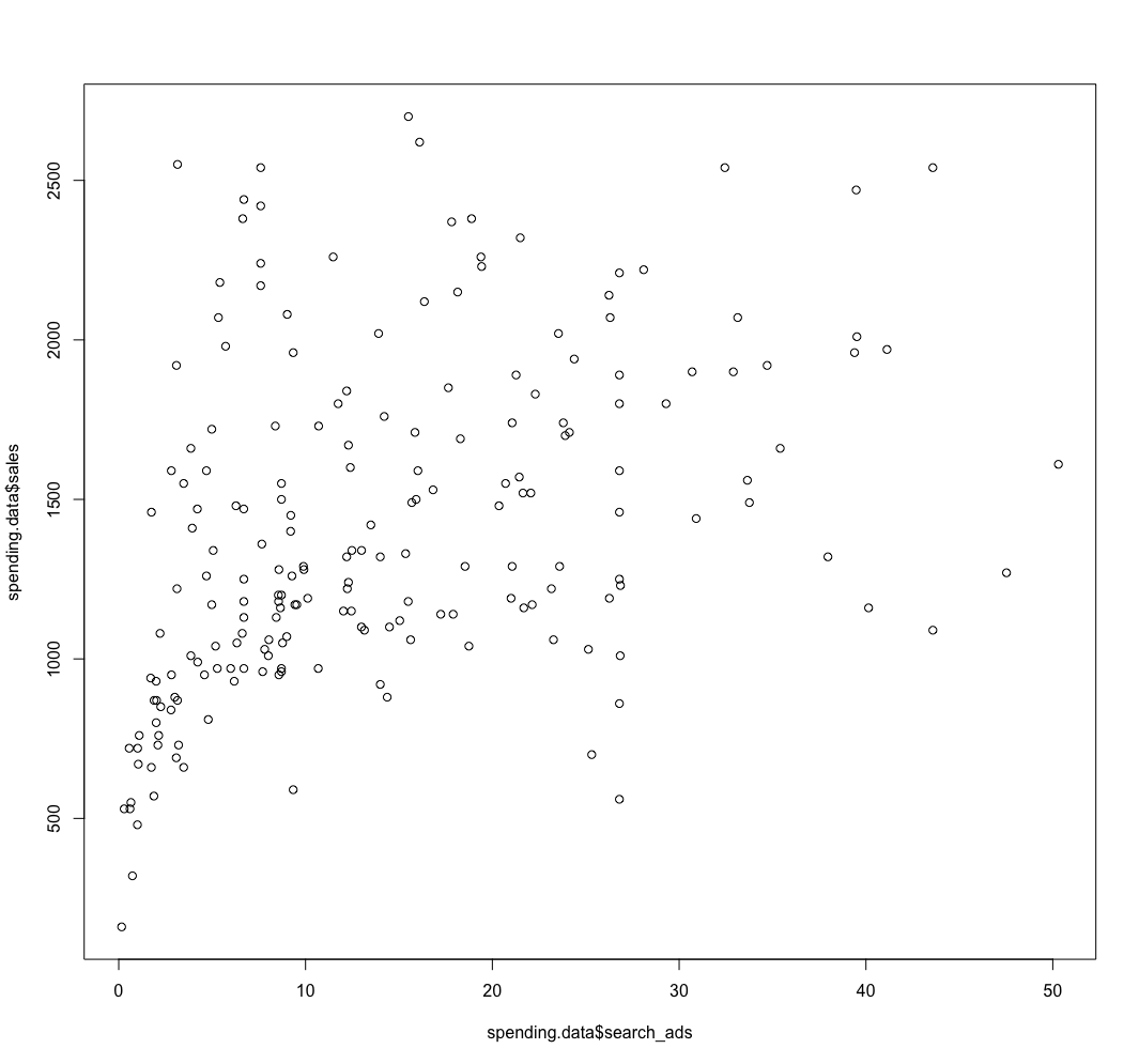
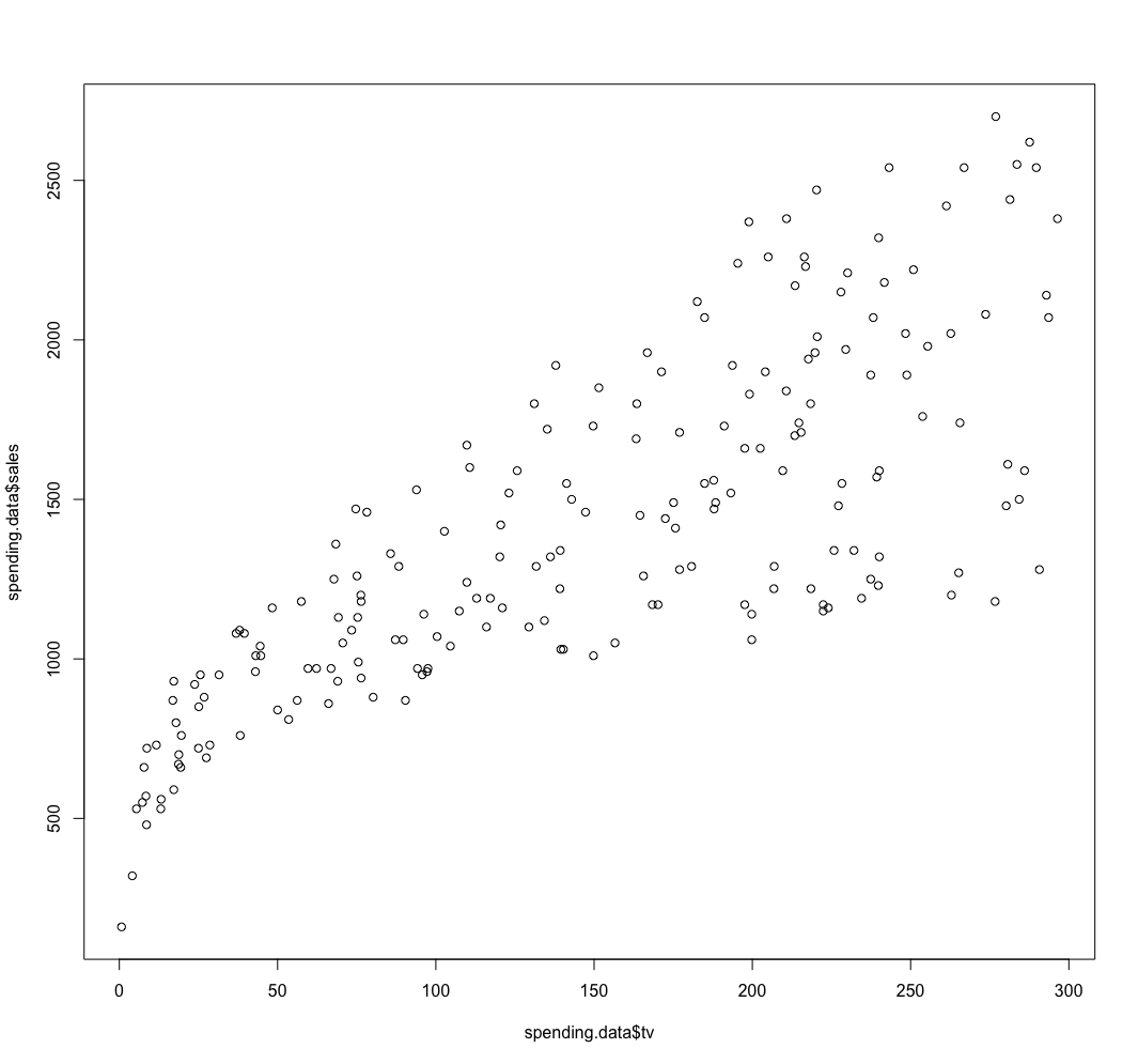
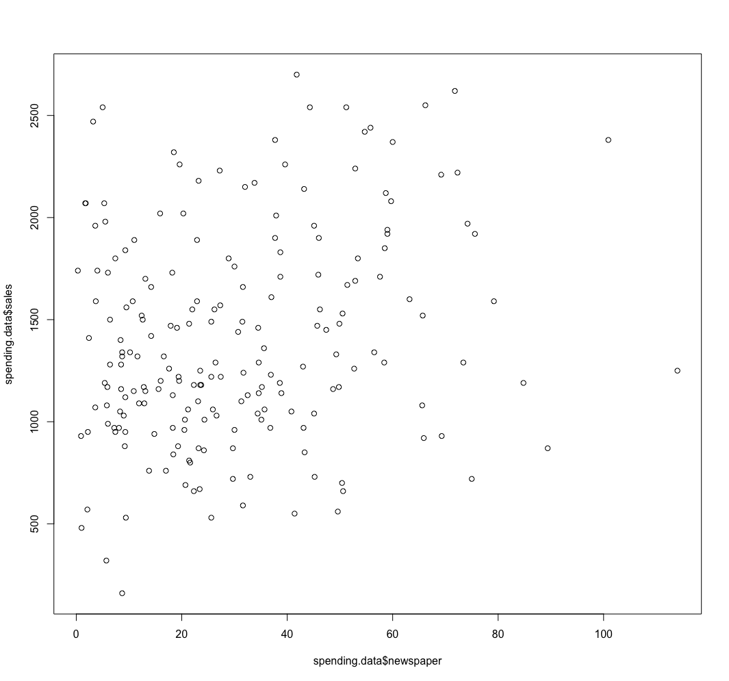
> ## log
> summary(spending.data$radio)
Min. 1st Qu. Median Mean 3rd Qu. Max.
0.04 9.30 22.00 23.23 36.35 79.60
> summary(spending.data$magazines)
Min. 1st Qu. Median Mean 3rd Qu. Max.
0.030 1.050 3.420 4.828 6.383 61.160
> summary(spending.data$social_media)
Min. 1st Qu. Median Mean 3rd Qu. Max.
0.245 7.050 18.137 22.289 33.523 90.800
> summary(spending.data$search_ads)
Min. 1st Qu. Median Mean 3rd Qu. Max.
0.1568 5.6442 11.6133 14.2485 21.4547 50.3014
> summary(spending.data$tv)
Min. 1st Qu. Median Mean 3rd Qu. Max.
0.70 74.38 149.75 147.04 218.82 296.40
> summary(spending.data$newspaper)
Min. 1st Qu. Median Mean 3rd Qu. Max.
0.30 12.75 25.75 30.55 45.10 114.00
>
> regression_2 <- lm(log(sales) ~ log(radio) + log(magazines) + log(social_media) + log(search_ads) + log(tv) + log(newspaper), data=spending.data)
> # 90.15% explained
> summary(regression_2)

Call:
lm(formula = log(sales) ~ log(radio) + log(magazines) + log(social_media) +
log(search_ads) + log(tv) + log(newspaper), data = spending.data)

Residuals:
Min 1Q Median 3Q Max
-0.53768 -0.08809 -0.01695 0.07090 0.58515

Coefficients:
Estimate Std. Error t value Pr(>|t|)
(Intercept) 5.066700 0.063064 80.342 <2e-16 ***
log(radio) 0.143520 0.008449 16.986 <2e-16 ***
log(magazines) 0.016958 0.015932 1.064 0.2885
log(social_media) 0.024575 0.015334 1.603 0.1107
log(search_ads) -0.037193 0.016400 -2.268 0.0244 *
log(tv) 0.364471 0.013843 26.329 <2e-16 ***
log(newspaper) 0.001954 0.017739 0.110 0.9124
---
Signif. codes: 0 ‘***’ 0.001 ‘**’ 0.01 ‘*’ 0.05 ‘.’ 0.1 ‘ ’ 1

Residual standard error: 0.13 on 193 degrees of freedom
Multiple R-squared: 0.9045, Adjusted R-squared: 0.9015
F-statistic: 304.7 on 6 and 193 DF, p-value: < 2.2e-16

3.1.2.3 log better

> regression <- lm(log(sales) ~ log(radio) + log(tv), data=spending.data) 
> # 89.93% explained
> summary(regression)

Call:
lm(formula = log(sales) ~ log(radio) + log(tv), data = spending.data)

Residuals:
Min 1Q Median 3Q Max
-0.53810 -0.09115 -0.01295 0.06795 0.58926

Coefficients:
Estimate Std. Error t value Pr(>|t|)
(Intercept) 5.098303 0.050058 101.85 <2e-16 ***
log(radio) 0.146733 0.008299 17.68 <2e-16 ***
log(tv) 0.356862 0.009271 38.49 <2e-16 ***
---
Signif. codes: 0 ‘***’ 0.001 ‘**’ 0.01 ‘*’ 0.05 ‘.’ 0.1 ‘ ’ 1

Residual standard error: 0.1315 on 197 degrees of freedom
Multiple R-squared: 0.9003, Adjusted R-squared: 0.8993
F-statistic: 889.6 on 2 and 197 DF, p-value: < 2.2e-16

3.1.3 Allocating Marketing Budget

Sum elasticity

0.49 = 0.14 + 0.35

Ratio of elasticity

0.2857 = 0.14 / 0.49

TV of elasticity

0.7143 = 0.35 / 0.49

Obtain elasticities from model

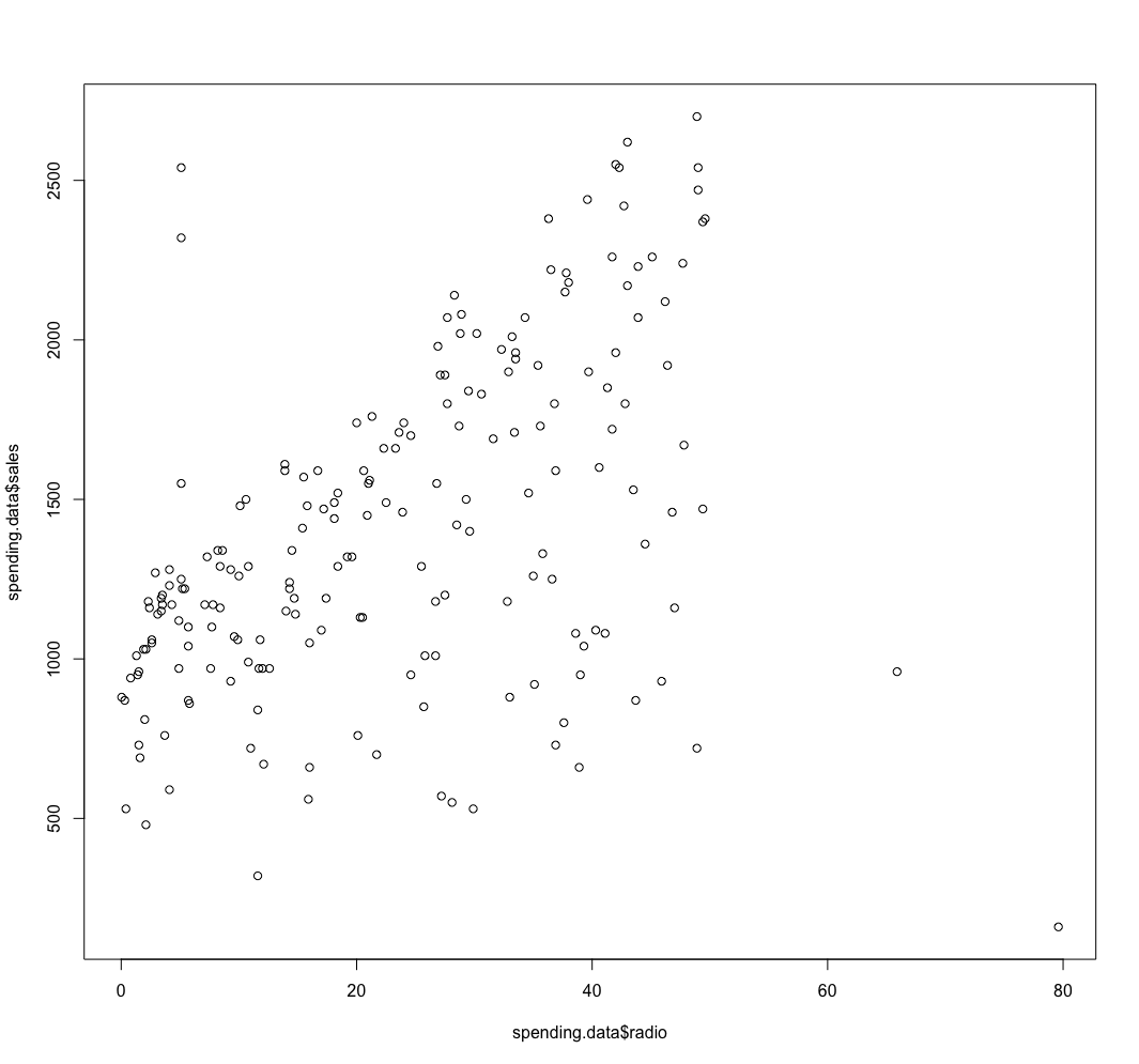
> mean(spending.data$radio)
[1] 23.2297
> mean(spending.data$tv)
[1] 147.0425
> mean(spending.data$sales)
[1] 1402.25
>
> # radio
> # A 1% increase in radio advertising results in a 0.26% increase in sales.
> 0.143520 * (23.2297 / 1402.25)
[1] 0.002377555
>
> # tv
> # A 1% increase in tv advertising results in a 0.26% increase in sales.
> 0.364471 * (147.0425 / 1402.25)
[1] 0.0382191

3.1.4 Advertising Carryover Effect

We are assumed to retain a 10% of your previous advertising stock.

> adstock <- function(x, rate){
+ return(as.numeric(stats::filter(x=x, filter=rate, method="recursive")))
+ }
>
> spending.data <- spending.data %>% mutate(tv_adstock = adstock(tv,0.1),
+ magazines_adstock = adstock(magazines, 0.1),
+ social_media_adstock = adstock(social_media, 0.1),
+ search_ads_adstock = adstock(search_ads, 0.1),
+ newspaper_adstock = adstock(newspaper, 0.1),
+ radio_adstock = adstock(radio, 0.1))
>
> regression_with_stock <- lm(log(sales) ~ log(radio_adstock) + log(magazines_adstock) + log(social_media_adstock) + log(search_ads_adstock) + log(tv_adstock) + log(newspaper_adstock), data=spending.data)
> # 90.15% explained
> summary(regression_with_stock)

Call:
lm(formula = log(sales) ~ log(radio_adstock) + log(magazines_adstock) +
log(social_media_adstock) + log(search_ads_adstock) + log(tv_adstock) +
log(newspaper_adstock), data = spending.data)

Residuals:
Min 1Q Median 3Q Max
-1.08867 -0.06993 0.00508 0.06916 0.53508

Coefficients:
Estimate Std. Error t value Pr(>|t|)
(Intercept) 4.253505 0.098083 43.366 <2e-16 ***
log(radio_adstock) 0.186030 0.013809 13.472 <2e-16 ***
log(magazines_adstock) 0.010671 0.019567 0.545 0.5861
log(social_media_adstock) 0.018066 0.020384 0.886 0.3766
log(search_ads_adstock) -0.040954 0.022445 -1.825 0.0696 .
log(tv_adstock) 0.484510 0.019831 24.432 <2e-16 ***
log(newspaper_adstock) 0.009142 0.023393 0.391 0.6964
---
Signif. codes: 0 ‘***’ 0.001 ‘**’ 0.01 ‘*’ 0.05 ‘.’ 0.1 ‘ ’ 1

Residual standard error: 0.1566 on 193 degrees of freedom
Multiple R-squared: 0.8615, Adjusted R-squared: 0.8572
F-statistic: 200 on 6 and 193 DF, p-value: < 2.2e-16

> spending.data <- spending.data %>% mutate(tv_adstock = adstock(tv,0.1),
+ radio_adstock = adstock(radio, 0.1))
>
> regression_with_stock <- lm(log(sales) ~ log(radio_adstock) + log(tv_adstock), data=spending.data)
> # 85.65% explained
> summary(regression_with_stock)

Call:
lm(formula = log(sales) ~ log(radio_adstock) + log(tv_adstock),
data = spending.data)

Residuals:
Min 1Q Median 3Q Max
-1.09358 -0.07401 -0.00318 0.07187 0.59975

Coefficients:
Estimate Std. Error t value Pr(>|t|)
(Intercept) 4.30635 0.08387 51.34 <2e-16 ***
log(radio_adstock) 0.18899 0.01318 14.34 <2e-16 ***
log(tv_adstock) 0.47064 0.01503 31.30 <2e-16 ***
---
Signif. codes: 0 ‘***’ 0.001 ‘**’ 0.01 ‘*’ 0.05 ‘.’ 0.1 ‘ ’ 1

Residual standard error: 0.157 on 197 degrees of freedom
Multiple R-squared: 0.858, Adjusted R-squared: 0.8565
F-statistic: 594.9 on 2 and 197 DF, p-value: < 2.2e-16

3.1.5 Synergy Effect

> # synergy effect
> center <- function(x) { scale(x, scale = F)}
>
> regression <- lm(log(sales) ~ log(radio) + log(magazines) + log(social_media) + log(search_ads) + log(tv) + log(newspaper) + log(radio) * log(tv), data=spending.data)
> summary(regression)

Call:
lm(formula = log(sales) ~ log(radio) + log(magazines) + log(social_media) +
log(search_ads) + log(tv) + log(newspaper) + log(radio) *
log(tv), data = spending.data)

Residuals:
Min 1Q Median 3Q Max
-0.29003 -0.07859 -0.02022 0.04670 0.54257

Coefficients:
Estimate Std. Error t value Pr(>|t|)
(Intercept) 5.880586 0.111464 52.758 < 2e-16 ***
log(radio) -0.117384 0.032064 -3.661 0.000325 ***
log(magazines) 0.026573 0.013728 1.936 0.054378 .
log(social_media) 0.029733 0.013181 2.256 0.025215 *
log(search_ads) -0.034111 0.014086 -2.422 0.016386 *
log(tv) 0.182792 0.024784 7.375 4.79e-12 ***
log(newspaper) -0.007208 0.015271 -0.472 0.637475
log(radio):log(tv) 0.058409 0.006992 8.354 1.30e-14 ***
---
Signif. codes: 0 ‘***’ 0.001 ‘**’ 0.01 ‘*’ 0.05 ‘.’ 0.1 ‘ ’ 1

Residual standard error: 0.1116 on 192 degrees of freedom
Multiple R-squared: 0.93, Adjusted R-squared: 0.9274
F-statistic: 364.2 on 7 and 192 DF, p-value: < 2.2e-16

>
> regression <- lm(log(sales) ~ log(radio) + log(tv) + log(radio) * log(tv), data=spending.data)
> summary(regression)

Call:
lm(formula = log(sales) ~ log(radio) + log(tv) + log(radio) *
log(tv), data = spending.data)

Residuals:
Min 1Q Median 3Q Max
-0.29435 -0.07741 -0.02310 0.05873 0.59461

Coefficients:
Estimate Std. Error t value Pr(>|t|)
(Intercept) 5.870204 0.104963 55.926 < 2e-16 ***
log(radio) -0.108507 0.032403 -3.349 0.000974 ***
log(tv) 0.184361 0.022818 8.080 6.53e-14 ***
log(radio):log(tv) 0.057335 0.007097 8.079 6.54e-14 ***
---
Signif. codes: 0 ‘***’ 0.001 ‘**’ 0.01 ‘*’ 0.05 ‘.’ 0.1 ‘ ’ 1

Residual standard error: 0.1142 on 196 degrees of freedom
Multiple R-squared: 0.9252, Adjusted R-squared: 0.9241
F-statistic: 808.3 on 3 and 196 DF, p-value: < 2.2e-16

>
> spending.data <- spending.data %>% mutate(radio_log_centered = center(log(radio)),
+ tv_log_centered = center(log(tv)),
+ newspaper_log_centered = center(log(newspaper)),
+ magazines_log_centered = center(log(magazines)),
+ social_media_log_centered = center(log(social_media)),
+ search_ads_log_centered = center(log(search_ads)))
>
> regression <- lm(log(sales) ~ radio_log_centered + magazines_log_centered + social_media_log_centered + search_ads_log_centered + tv_log_centered + newspaper_log_centered + radio_log_centered * tv_log_centered, data=spending.data)
> summary(regression)

Call:
lm(formula = log(sales) ~ radio_log_centered + magazines_log_centered +
social_media_log_centered + search_ads_log_centered + tv_log_centered +
newspaper_log_centered + radio_log_centered * tv_log_centered,
data = spending.data)

Residuals:
Min 1Q Median 3Q Max
-0.29003 -0.07859 -0.02022 0.04670 0.54257

Coefficients:
Estimate Std. Error t value Pr(>|t|)
(Intercept) 7.169892 0.007894 908.260 < 2e-16 ***
radio_log_centered 0.155506 0.007395 21.027 < 2e-16 ***
magazines_log_centered 0.026573 0.013728 1.936 0.0544 .
social_media_log_centered 0.029733 0.013181 2.256 0.0252 *
search_ads_log_centered -0.034111 0.014086 -2.422 0.0164 *
tv_log_centered 0.343443 0.012150 28.267 < 2e-16 ***
newspaper_log_centered -0.007208 0.015271 -0.472 0.6375
radio_log_centered:tv_log_centered 0.058409 0.006992 8.354 1.3e-14 ***
---
Signif. codes: 0 ‘***’ 0.001 ‘**’ 0.01 ‘*’ 0.05 ‘.’ 0.1 ‘ ’ 1

Residual standard error: 0.1116 on 192 degrees of freedom
Multiple R-squared: 0.93, Adjusted R-squared: 0.9274
F-statistic: 364.2 on 7 and 192 DF, p-value: < 2.2e-16

>
> regression <- lm(log(sales) ~ radio_log_centered + tv_log_centered + radio_log_centered * tv_log_centered, data=spending.data)
> summary(regression)

Call:
lm(formula = log(sales) ~ radio_log_centered + tv_log_centered +
radio_log_centered * tv_log_centered, data = spending.data)

Residuals:
Min 1Q Median 3Q Max
-0.29435 -0.07741 -0.02310 0.05873 0.59461

Coefficients:
Estimate Std. Error t value Pr(>|t|)
(Intercept) 7.169879 0.008074 888.050 < 2e-16 ***
radio_log_centered 0.159367 0.007374 21.611 < 2e-16 ***
tv_log_centered 0.342059 0.008256 41.429 < 2e-16 ***
radio_log_centered:tv_log_centered 0.057335 0.007097 8.079 6.54e-14 ***
---
Signif. codes: 0 ‘***’ 0.001 ‘**’ 0.01 ‘*’ 0.05 ‘.’ 0.1 ‘ ’ 1

Residual standard error: 0.1142 on 196 degrees of freedom
Multiple R-squared: 0.9252, Adjusted R-squared: 0.9241
F-statistic: 808.3 on 3 and 196 DF, p-value: < 2.2e-16

3.2 Compare groups

3.2.1 import and check data

> ad.df <- read.csv("8_clickstream.csv", stringsAsFactors = TRUE) 
> summary(ad.df)
visit_date condition time_spent_homepage_sec clicked_article
13/04/2020: 1045 quality:15000 Min. :46.10 Min. :0.0000
23/04/2020: 1042 taste :15000 1st Qu.:49.32 1st Qu.:0.0000
02/04/2020: 1038 Median :50.00 Median :1.0000
31/03/2020: 1033 Mean :50.00 Mean :0.6054
15/04/2020: 1031 3rd Qu.:50.67 3rd Qu.:1.0000
27/04/2020: 1029 Max. :54.02 Max. :1.0000
(Other) :23782
clicked_like clicked_share
Min. :0.0000 Min. :0.00000
1st Qu.:0.0000 1st Qu.:0.00000
Median :0.0000 Median :0.00000
Mean :0.1177 Mean :0.03143
3rd Qu.:0.0000 3rd Qu.:0.00000
Max. :1.0000 Max. :1.00000

> str(ad.df)
'data.frame': 30000 obs. of 6 variables:
$ visit_date : Factor w/ 30 levels "01/04/2020","02/04/2020",..: 30 30 30 30 30 30 30 30 30 30 ...
$ condition : Factor w/ 2 levels "quality","taste": 2 2 2 2 2 2 2 2 2 2 ...
$ time_spent_homepage_sec: num 49 48.9 49.1 49.3 50.4 ...
$ clicked_article : int 1 1 1 0 0 1 1 1 1 0 ...
$ clicked_like : int 0 0 0 1 1 0 0 0 0 0 ...
$ clicked_share : int 1 0 0 0 0 0 0 0 0 0 ...

> ad.df$clicked_article <- factor(ad.df$clicked_article, ordered = FALSE)
> ad.df$clicked_like <- factor(ad.df$clicked_like, ordered = FALSE)
> ad.df$clicked_share <- factor(ad.df$clicked_share, ordered = FALSE)

3.2.2 Descriptives by group

3.2.2.1 seconds spent vary for two versions of ads.

> # seconds spent vary for two versions of ads.
> aggregate(time_spent_homepage_sec ~ condition, data = ad.df, mean)
condition time_spent_homepage_sec
1 quality 49.99489
2 taste 49.99909

3.2.2.2 the frequency with which different combinations of condition and like occur

> table(ad.df$condition, ad.df$clicked_article)

0 1
quality 5873 9127
taste 5965 9035
> table(ad.df$condition, ad.df$clicked_like)

0 1
quality 13964 1036
taste 12506 2494
> table(ad.df$condition, ad.df$clicked_share)

0 1
quality 14550 450
taste 14507 493

3.2.3 Visualization by group

> histogram(~ clicked_article | condition, data = ad.df)
> histogram(~ clicked_like | condition, data = ad.df)
> histogram(~ clicked_share | condition, data = ad.df)
> ad.mean <- aggregate(time_spent_homepage_sec ~ condition, data = ad.df, mean) 
> barchart(time_spent_homepage_sec ~ condition, data = ad.mean, col = "grey")

3.2.4 Statistical tests

3.2.4.1 chisp.test()

> # chisp.test()
> chisq.test(table(ad.df$clicked_article, ad.df$condition))

Pearson's Chi-squared test with Yates' continuity correction

data: table(ad.df$clicked_article, ad.df$condition)
X-squared = 1.1555, df = 1, p-value = 0.2824

> chisq.test(table(ad.df$clicked_like, ad.df$condition))

Pearson's Chi-squared test with Yates' continuity correction

data: table(ad.df$clicked_like, ad.df$condition)
X-squared = 681.57, df = 1, p-value < 2.2e-16

> chisq.test(table(ad.df$clicked_share, ad.df$condition))

Pearson's Chi-squared test with Yates' continuity correction

data: table(ad.df$clicked_share, ad.df$condition)
X-squared = 1.9313, df = 1, p-value = 0.1646

3.2.4.2 t.test()

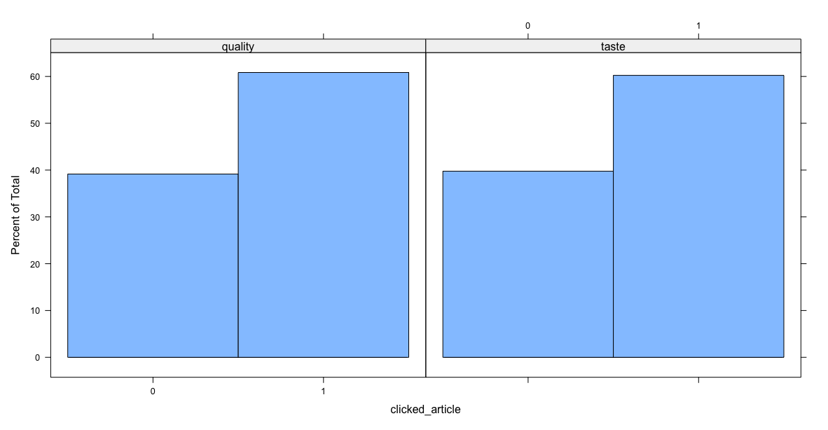
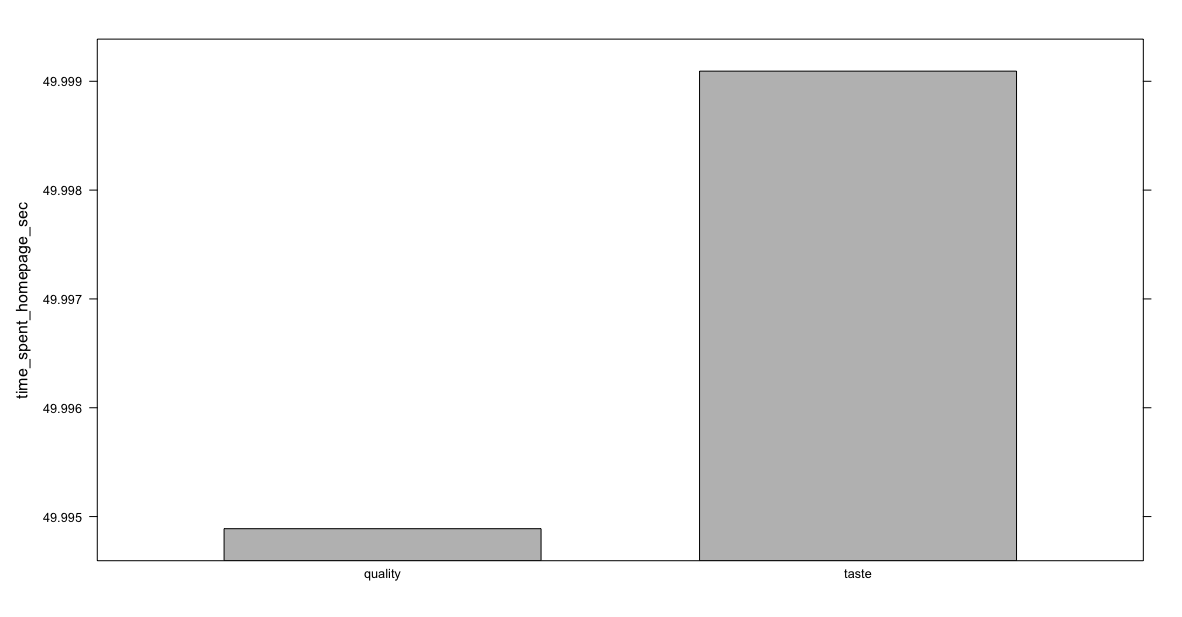
> # t.test()
> t.test(time_spent_homepage_sec ~ condition, data = ad.df)

Welch Two Sample t-test

data: time_spent_homepage_sec by condition
t = -0.36288, df = 29997, p-value = 0.7167
alternative hypothesis: true difference in means between group quality and group taste is not equal to 0
95 percent confidence interval:
-0.02691480 0.01850573
sample estimates:
mean in group quality mean in group taste
49.99489 49.99909

3.2.4.3 anova

> ad.aov.con <- aov(time_spent_homepage_sec ~ condition, data = ad.df)
> anova(ad.aov.con)
Analysis of Variance Table

Response: time_spent_homepage_sec
Df Sum Sq Mean Sq F value Pr(>F)
condition 1 0.1 0.13259 0.1317 0.7167
Residuals 29998 30204.2 1.00687